Lecture 3

Today

• Kohn-Sham equations

• Density response and screening

• Response functions

Reading

GY: 15.5--15.7.

Giuliani and Vignale. Quantum Theory of the Electron Liquids. 3.2.1 -- 3.2.7, 3.3.1 -- 3.3.5.

1. The Kohn-Sham equations

• The Kohn-Sham Lagrangian

The DFT variational principle means

Note

and

where the exchange-correlation potential is defined as

is the functional derivative of the exchange-correlation energy functional with respect to density, called

Then we arrive at the Kohn-Sham equations

The only assumption up to this point is the non-interacting v-representability, which is justifiable to a great extent. Note that the eigenvalues ${\epsilon }_i$$\varepsilon_i$ are understood to be the Lagrange multipliers (拉格朗日乘子), which unlike the counterparts in Hartree-Fock approximation have no clear physical meaning.

However, the K-S equations are useless yet, because $E_{\text{xc}}$$E_{\text{xc}}$ and $v_{\text{xc}}$$v_{\text{xc}}$ are unknown. In order to make these equations useful, one has to make various local approximations, as explained in the textbook.

2. Density response

• Density is the key variable, as we have demonstrated in the density functional theory.

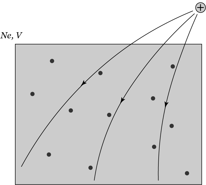
• Adding external charge/potential to a many-electron system

  

• From the DFT, we have

  $$\begin{array}{}\text{(5)}& E[n]=E_{\text{int}}[n]+\int {\text{d}}^{3}r{v}_{\text{ext}}(\mathit{r})n(\mathit{r})\end{array}$$

  Let $n_0$$n_0$ be the g.s. density of the many-electron system without $v_{\text{ext}}$$v_{\text{ext}}$. Performing a functional expansion of $E_{\text{int}}$$E_\text{int}$ around $n_0$$n_0$

  $$\begin{array}{}\text{(6)}& E_{\text{int}}[n]=E_{\text{int}}[n_0]+\frac{1}{2}\int {\text{d}}^{3}r\int {\text{d}}^3{r}^{\prime }\delta n(\mathit{r})\delta n({\mathit{r}}^{\prime }){\left[\frac{{\delta }^2{E}_{\text{int}}}{\delta n(\mathit{r})\delta n({\mathit{r}}^{\prime })}\right]}_{n=n_0}+\cdots \end{array}$$

  If we are to reach a new stable state in the external potential, we need

  $$\begin{array}{}\text{(7)}& \frac{\delta E}{\delta n(\mathit{r})}=\int {\text{d}}^3{r}^{\prime }\delta n({\mathit{r}}^{\prime }){\left[\frac{{\delta }^2{E}_{\text{int}}}{\delta n(\mathit{r})\delta n({\mathit{r}}^{\prime })}\right]}_{n=n_0}+v_{\text{ext}}(\mathit{r})=0\end{array}$$

  this means

  $$\begin{array}{}\text{(8)}& \delta n(\mathit{r})=\int {\text{d}}^3{r}^{\prime }\chi (\mathit{r},{\mathit{r}}^{\prime })v_{\text{ext}}({\mathit{r}}^{\prime })\end{array}$$

  we have introduced the static density response function (or susceptibility) as the functional inverse

  $$\begin{array}{}\text{(9)}& \chi (\mathit{r},{\mathit{r}}^{\prime })=-{\left\{{\left[\frac{{\delta }^2{E}_{\text{int}}}{\delta n(\mathit{r})\delta n({\mathit{r}}^{\prime })}\right]}_{n=n_0}\right\}}^{-1}\end{array}$$

  The functional inverse of a two-point function $A(\mathit{r},{\mathit{r}}^{\prime })$$A(\boldsymbol r,\boldsymbol r')$ is defined by analogy with the matrix inverse

  $$\begin{array}{}\text{(10)}& \int {\text{d}}^3{r}^{″}A(\mathit{r},{\mathit{r}}^{″})A^{-1}({\mathit{r}}^{″},{\mathit{r}}^{\prime })=\delta (\mathit{r}-{\mathit{r}}^{\prime })\end{array}$$

• Now we calculate the susceptibility for an interacting many-electron system

Noting that w/o interaction

Putting together, we find

• Now for a uniform system (like the electron gas), $\chi (\mathit{r},{\mathit{r}}^{\prime })=\chi (\mathit{r}-{\mathit{r}}^{\prime })$$\chi(\boldsymbol r,\boldsymbol r') =\chi(\boldsymbol r-\boldsymbol r')$. Its Fourier transform is

  $$\begin{array}{}\text{(14)}& \begin{array}{c}\chi (\mathit{q})=\int {\text{d}}^{3}r{e}^{-\mathrm{i}\mathit{q}\cdot \mathit{r}}\chi (\mathit{r})\\ \chi (\mathit{r})=\int [\text{d}q]e^{\mathrm{i}\mathit{q}\cdot \mathit{r}}\chi (\mathit{q}).\end{array}\end{array}$$

  Thus

  $$\begin{array}{}\text{(15)}& \delta n(\mathit{q})=\chi (\mathit{q})v_{\text{ext}}(\mathit{q})\end{array}$$

  Then the susceptibility is

  $$\begin{array}{}\text{(16)}& \begin{array}{rl}-{\chi }^{-1}(\mathit{q})& =-{\chi }_0^{-1}(\mathit{q})+v_c(\mathit{q})+F_{\text{xc}}(\mathit{q})\\ & =v_{\text{c}}(\mathit{q})-{\mathrm{\Pi }}^{-1}(\mathit{q})\end{array}\end{array}$$

  where the polarization function $\mathrm{\Pi }$$\Pi$ is defined as

  $$\begin{array}{}\text{(17)}& {\mathrm{\Pi }}^{-1}(\mathit{q})={\chi }_0^{-1}(\mathit{q})-F_{\text{xc}}(\mathit{q})\end{array}$$

3. Screening

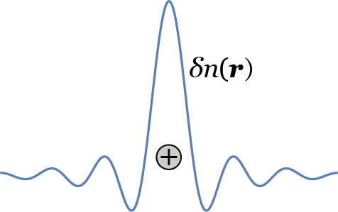
• Screening occurs when the potential from the induced charge is superimposed on the original (external) potential.

where the (static) dielectric function is defined as

• Example: Thomas-Fermi approximation. Let $\mathrm{\Pi }={\chi }_0$$\Pi = \chi_0$, i.e. ignoring $F_{\text{xc}}$$F_{\text{xc}}$.

  $$\begin{array}{}\text{(20)}& \chi (\mathit{q})=\frac{{\chi }_0(\mathit{q})}{1-v_{\text{c}}(\mathit{q}){\chi }_0(\mathit{q})}\end{array}$$

  Thomas-Fermi: ${\chi }_0(\mathit{q})={\chi }_0(0)$$\chi_0(\boldsymbol q) = \chi_0(0)$. Recall in S.I.

  $$\begin{array}{}\text{(21)}& v_{\text{c}}(q)=\frac{e^2}{{ϵ}_0{q}^2}\end{array}$$

  we define the Thomas-Fermi wavevector (托马斯-费米波矢)

  $$\begin{array}{}\text{(22)}& q_{\text{TF}}^2=-\frac{e^2}{{ϵ}_0}{\chi }_0(0)\end{array}$$

  Then in the T-F approximation,

  $$\begin{array}{}\text{(23)}& \chi (q)=\frac{{\chi }_0(0)}{1+q_{\text{TF}}^2/q^2}\end{array}$$

  • what is ${\chi }_0(q)$$\chi_0(q)$ in the long-wavelength limit (长波极限)?

    $$\begin{array}{}& \begin{array}{c}\begin{array}{rl}\delta n(\mathit{r})& =\int {\text{d}}^3{r}^{\prime }{\chi }_0(\mathit{r}-{\mathit{r}}^{\prime })v_{\text{ext}}({\mathit{r}}^{\prime })\\ & =\int [\text{d}q]e^{\mathrm{i}\mathit{q}\cdot \mathit{r}}{\chi }_0(\mathit{q})v_{\text{ext}}(\mathit{q})\\ & \approx {\chi }_0(q=0)v_{\text{ext}}(\mathit{r})\end{array}\end{array}\end{array}$$

    That is,

    $$\begin{array}{}\text{(24)}& {\chi }_0(0)=\frac{\partial n}{\partial v}=-\frac{\partial n}{\partial \mu }=-g_s{g}_0\end{array}$$

    where $g_0$$g_0$ is the density of state at the Fermi level per spin, and $g_s=2$$g_s=2$ is the spin degeneracy factor.

  • Then in the T-F approximation,

    $$\begin{array}{}\text{(25)}& \begin{array}{c}{v}_{\text{TF}}(\mathit{q})=(1+v_{\text{c}}(q)\chi (q))v_{\text{ext}}(\mathit{q})\\ =\frac{v_{\text{ext}}(\mathit{q})}{1-v_c(q){\chi }_0(q)}\\ =\frac{v_{\text{ext}}(\mathit{q})}{1+q_{\text{TF}}^2/q^2}\end{array}\end{array}$$

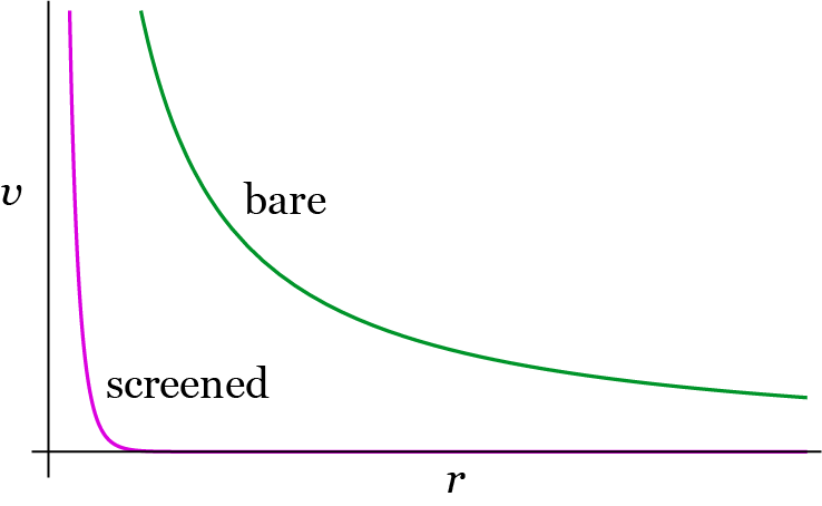
    So for a point charge, the external potential it produces is

    $$\begin{array}{}\text{(26)}& \begin{array}{c}{v}_{\text{TF}}(q)=\frac{e^2}{{ϵ}_0(q^2+q_{\text{TF}}^2)}\\ v_{\text{TF}}(r)=\frac{e^2}{4\pi {ϵ}_{0}r}{e}^{-q_{\text{TF}}r}\end{array}\end{array}$$

    This is the screened Coulomb potential within the Thomas-Fermi approximation. As shown in the Figure below, the bare Coulomb interaction is long-ranged. But in a many-body system, the restructuring of charge in an external potential (even without considering the interactions between electrons) lead to induced charges $-e\delta n(\mathit{r})$$-e\delta n(\boldsymbol r)$ that screen out the external charge, resulting in a short-ranged potential.

    

4. Linear response theory

How do we compute the $\chi$$\chi$ for a many-electron system, in general? The theoretical machinery is the linear response theory. The idea is the following. All local measurements on a quantum many-body system amounts to a process of response at $({\mathit{r}}^{\prime },t^{\prime })$$(\boldsymbol r',t')$ to an earlier disturbance at $(\mathit{r},t)$$(\boldsymbol r,t )$. As it will be shown, the microscopic process leading such responses can be broken down into some basic types of excitations in the many-body system. What is more surprising, is that the responses as a kinetic process has very simple relations to the correlation of fluctuation in the equilibrium ensemble.

When we talk of some disturbance to a system, it is an external field $F(t)$$F(t)$ (e.g., electromagnetic¹) that couples to some internal degree of freedom (charge, spin, etc.), say $B$$B$, through

We will assume that the perturbation is weak, such that a perturbation theory is justified. The question we will try to answer is: how a variable of the system evolves when the perturbation is turned on at $t=0$$t=0$.

We approach the problem using the quantum Liouville /ˌliːuːˈvɪl/ equation

We will be working in the grand canonical ensemble

In the interaction picture, the density operator is

the equation of motion (EOM 运动方程) is calculated as

This is a first-order operator equation, whose solution is formally

Again, this is a fixed-point problem. Truncating at the first iteration, we have

Now for an observable $A$$A$, the dynamics is given by

So we obtain the retarded linear response function

so that

The correlation function describes, when a disturbance is introduced to a many-electron system by coupling to $B$$B$, how the dynamics of the system prescribes the evolution of $A$$A$. The Heaviside step function $\theta (t-t^{\prime })$$\theta(t-t')$ means that the response of $A$$A$ is determined by an earlier disturbance coupled to $B$$B$, reflecting causality (因果性). Therefore, ${\chi }_{AB}(t-t^{\prime })$$\chi_{AB}(t-t')$ is called the retarded (推迟的) or causal response function.