Lecture 4

03/02/23, Th.

Today

Response functions of a noninteracting system.
Lindhard function and its structure.

Reading

GY 15.7-15.9.
Giuliani and Vignale. Quantum Theory of the Electron Liquids. 4.1- 4.4.

1. Non-interacting system

\begin{matrix} (1) & H_{0} = \sum_{α} ε_{α} a_{α}^{†} a_{α} \end{matrix}

The observables

\begin{matrix} (2) & \begin{matrix} A = \sum_{α β} A_{α β} a_{α}^{†} a_{β} \\ B = \sum_{α β} B_{α β} a_{α}^{†} a_{β} \end{matrix} \end{matrix}

Then

\begin{matrix} χ_{A B}^{0} (t) = - \frac{i}{ℏ} θ (t) \sum_{α β γ η} A_{α β} B_{γ η} ⟨ [a_{α}^{†} (t) a_{β} (t), a_{γ}^{†} a_{η}] ⟩_{0} \end{matrix}

Noting the identity

\begin{matrix} [a_{α}^{†} a_{β}, a_{γ}^{†} a_{η}] = δ_{β γ} a_{α}^{†} a_{η} - δ_{α η} a_{γ}^{†} a_{β} \end{matrix}

We find

\begin{matrix} (3) & χ_{A B}^{0} (t) = - \frac{i}{ℏ} θ (t) \sum_{α β} A_{α β} B_{β α} (f_{0} (ε_{α}) - f_{0} (ε_{β})) e^{i (ε_{α} - ε_{β}) t / ℏ} \end{matrix}

In the frequency domain

\begin{matrix} (4) & χ_{A B}^{0} (ω) = \int_{- \infty}^{\infty} d t e^{i ω^{+} t} χ_{A B}^{0} (0) = \sum_{α β} A_{α β} B_{β α} \frac{f_{0} (ε_{α}) - f_{0} (ε_{β})}{ℏ ω + ε_{α} - ε_{β} + i 0^{+}} \end{matrix}

where

\begin{matrix} (5) & ω^{+} = ω + i 0^{+} . \end{matrix}

$\mathrm i 0^+$ $H_0$ $\chi^0_{AB}(\omega)$ then describes the response to a periodic perturbation like

\begin{matrix} (6) & F (r, t) = F e^{i (q \cdot r - ω t)} + F^{*} e^{- i (q \cdot r - ω t)} \end{matrix}

so that

\begin{matrix} (7) & δ A (ω) = χ_{A B}^{0} (ω) F \end{matrix}

Next, we consider the density response function. The density operator is

\begin{matrix} \begin{matrix} \begin{aligned} n (r) & = \sum_{σ} ψ_{σ}^{†} (r) ψ_{σ} (r) \\ = \frac{1}{V} \sum_{σ} \sum_{k} \sum_{k^{'}} a_{k σ}^{†} a_{k^{'} σ} e^{- i (k - k^{'}) \cdot r} \\ = \int [d q] e^{i q \cdot r} \sum_{σ} \sum_{k σ} a_{k σ}^{†} a_{k + q σ} \end{aligned} \end{matrix} \end{matrix}

\begin{matrix} (8) & n (q) = \sum_{k σ} a_{k σ}^{†} a_{k + q σ} \end{matrix}

Think of

\begin{matrix} \begin{matrix} \begin{aligned} δ n (r, t) & = - \frac{i}{ℏ} \int d^{3} r^{'} \int d t^{'} ⟨ [n (r, t), n (r^{'}, t^{'})] ⟩_{0} {F e^{i (q \cdot r^{'} - ω t^{'})} + c.c.} \\ = - \frac{i}{ℏ} \int d t^{'} θ (t - t^{'}) ⟨ [n (r, t), n (- q, - t^{'})] ⟩_{0} F + c.c. \end{aligned} \end{matrix} \end{matrix}

So for the density response commensurate with the external fields

\begin{matrix} (9) & δ n (q, t) = - \frac{i}{ℏ} \int d t^{'} θ (t - t^{'}) ⟨ [n (q, t), n (- q, - t^{'})] ⟩_{0} F \end{matrix}

This means

\begin{matrix} (10) & χ^{0} (q, t - t^{'}) = - \frac{i}{ℏ} θ (t - t^{'}) ⟨ [n (q, t), n (- q, t^{'})] ⟩_{0} \end{matrix}

So that

\begin{matrix} (11) & χ^{0} (q, ω) = \sum_{s} \int [d k] \frac{f_{0} (ε_{k s}) - f_{0} (ε_{k + q s})}{ℏ ω + ε_{k s} - ε_{k + q s} + i 0^{+}} \end{matrix}

This is the so-called Lindhard function.

Digression on spin response

$n_s(\boldsymbol r)$ $s,s' = \uparrow, \downarrow$ . We define the total density and spin polarization, respectively, as

\begin{matrix} (12) & \begin{matrix} n (r) = n_{↑} (r) + n_{↓} (r) \\ m (r) = n_{↑} (r) - n_{↓} (r) = S_{z} (r) \end{matrix} \end{matrix}

Then the spin-resolved density–density response function is defined as

\begin{matrix} (13) & χ_{s s^{'}} (r, r^{'}, t - t^{'}) = - \frac{i}{ℏ} ⟨ [n_{s} (r t), n_{s}^{'} (r^{'} t^{'})] ⟩ θ (t - t^{'}) \end{matrix}

Clearly,

\begin{matrix} (14) & χ_{n n} = \sum_{s s^{'}} χ_{s s^{'}} \end{matrix}

longitudinal $\delta m$ to the Zeeman field

\begin{matrix} (15) & χ_{S} = χ_{m m} = \sum_{s s^{'}} s s^{'} χ_{s s^{'}}, with s = \pm 1 for ↑ / ↓ . \end{matrix}

$χ_{↑↑} = χ_{↓↓}$ . Thus, spin and density responses are perfectly decoupled in a paramagnetic electron liquid: this is an exact result.

$\chi_{\uparrow \downarrow }=\chi_{ \downarrow \uparrow}=0$ .¹ So

\begin{matrix} (16) & χ_{S}^{0} (q, ω) = χ^{0} (q, ω) \end{matrix}

$\frac{\hbar}{2}$ ) is defined as

\begin{matrix} (17) & S^{α} (r) = \sum_{s s^{'}} ψ_{s}^{†} (r) σ_{s s^{'}}^{α} ψ (r) \end{matrix}

$\sigma^\alpha$ are the Pauli matrices

\begin{matrix} (18) & \begin{matrix} σ_{x} = (\begin{array}{ll} 0 & 1 \\ 1 & 0 \end{array}), σ_{y} = (\begin{array}{cc} 0 & - i \\ i & 0 \end{array}), σ_{z} = (\begin{array}{cc} 1 & 0 \\ 0 & - 1 \end{array}) . \end{matrix} \end{matrix}

which have following properties

\begin{matrix} (19) & σ^{α} σ^{β} = δ^{α β} + i \sum_{γ} ϵ^{α β γ} σ^{γ} . \end{matrix}

Additionally

\begin{matrix} (20) & σ^{\pm} = \frac{1}{2} (σ^{x} \pm i σ^{y}) \end{matrix}

\begin{matrix} (21) & S^{α} (q) = \sum_{k, s s^{'}} a_{k s}^{†} σ_{s s^{'}}^{α} a_{k + q s^{'}} \end{matrix}

$\chi_{S_+S_-}$ . For the non-interacting electron gas

\begin{matrix} (22) & χ_{S_{+} S_{-}}^{0} (q, ω) = \sum_{σ} \int [d k] \frac{f_{0} (ε_{k ↑}) - f_{0} (ε_{k + q ↓})}{ℏ ω + ε_{k ↑} - ε_{k + q ↓} + i 0^{+}} \end{matrix}

2. The Lindhard function

$\eqref{eq:lind}$ contains some essential information of how a many-electron system responds to external fields. We'd like to inspect its structure after analytically computing it. Since spin is good quantum number in this case, we can compute the spin Lindhard function defined as

\begin{matrix} (23) & χ_{s}^{0} (q, ω) = \int [d k] \frac{f_{0} (ε_{k s}) - f_{0} (ε_{k + q s})}{ℏ ω + ε_{k s} - ε_{k + q s} + i 0^{+}} . \end{matrix}

Now we separate the above into two sums over the occupied states

\begin{matrix} (24) & \begin{matrix} χ_{s}^{0} (q, ω) = \int [d k] \frac{f_{0} (ε_{k s})}{ℏ ω^{+} + ε_{k s} - ε_{k + q s}} \\ + \int [d k] \frac{f_{0} (ε_{k s})}{- ℏ ω^{+} + ε_{k s} - ε_{k + q s}} . \end{matrix} \end{matrix}

$\boldsymbol k \rightarrow -\boldsymbol k-\boldsymbol q$ .

Using the dispersion relation for a free-electron gas

\begin{matrix} \begin{matrix} \begin{aligned} \int [d k] \frac{f_{0} (ε_{k s})}{ℏ ω^{+} + ε_{k s} - ε_{k + q s}} \\ = \frac{m}{ℏ^{2} k_{F σ} q} \int [d k] \frac{f_{0} (ε_{k s})}{\frac{ω^{+}}{q v_{F s}} - \frac{q}{2 k_{F s}} - \frac{k}{k_{F s}} \cos θ} \\ [T = 0] & = \frac{m k_{F σ}^{d - 1}}{ℏ^{2} q} \int_{0}^{1} d x x^{d - 1} \int \frac{d Ω_{d}}{(2 π)^{d}} \frac{f_{0} (ε_{k s})}{\frac{ω^{+}}{q v_{F s}} - \frac{q}{2 k_{F s}} - x \cos θ} \end{aligned} \end{matrix} \end{matrix}

$\cos\theta = \hat{\boldsymbol k}\cdot\hat{\boldsymbol q}$ $x=x/k_{\text {Fs}}$ $\Omega_d$ $d$ -dimensions.

Now define a function

\begin{matrix} (25) & Ψ_{d} (z) \equiv \int_{0}^{1} d x x^{d - 1} \int \frac{d Ω_{d}}{Ω_{d}} \frac{1}{z - x \cos θ} \end{matrix}

$\Psi_d(-z)=-\Psi_d(z)$

We find

\begin{matrix} (26) & χ_{s}^{0} (q, ω) = \frac{g_{0 s} k_{F s}}{q} [Ψ_{d} (\frac{ω^{+}}{q v_{F σ}} - \frac{q}{2 k_{F σ}}) - Ψ_{d} (\frac{ω^{+}}{q v_{F σ}} + \frac{q}{2 k_{F σ}})] \end{matrix}

Table 4.1 from Electron Liquids.

$\omega =0$
$\begin{matrix} (27) & \begin{matrix} χ^{0} (q, ω) = \sum_{σ} \int [d k] \frac{f_{0} (ε_{k σ}) - f_{0} (ε_{k + q σ})}{ε_{k σ} - ε_{k + q σ}} \end{matrix} \end{matrix}$ $\begin{matrix} (28) & \begin{array}{ll} d = 3 : χ_{s}^{0} (q, 0) & = - g (0) [\frac{1}{2} - \frac{1 - x^{2}}{2 x} \log | \frac{x - 1}{x + 1} |] \\ d = 2 : χ_{s}^{0} (q, 0) & = - g (0) [1 - θ (x - 1) \sqrt{1 - \frac{1}{x^{2}}}] \\ d = 1 : χ_{s}^{0} (q, 0) & = - g (0) (\frac{1}{2 x} \log | \frac{x - 1}{x + 1} |) \end{array} \end{matrix}$

Static Lindhard functions for d=1,2,3. Lines are analytical results, and dots are from an adaptive MC integration

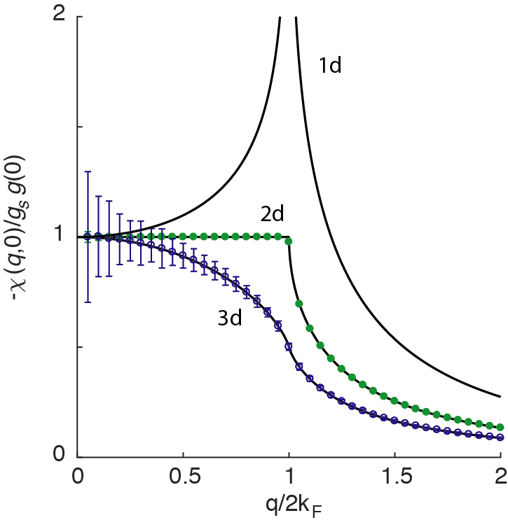
$q=2k_{\text F}$ $\chi^0$ diverges logarithmically for 1-dimensional system, and has discontinuity in the derivatives for 2- and 3-dimensional systems. A singularity in a function can produce long-range features in the Fourier spectrum, which in this case is the density variation in position space. It turns out, these integrals can be again evaluated analytically. Take the 3d case for example

\begin{matrix} (29) & χ^{0} (r, 0) = - 12 π n g (0) \frac{\sin (2 k_{F} r) - 2 k_{F} r \cos (2 k_{F} r)}{{(2 k_{F} r)}^{4}} \end{matrix}

$k_\text F^3 = 3\pi^2 n$ $\cos (2k_\text Fr)/r^3$ $r$ $π/k_\text F$ caused by external potential is called the Friedel oscillation.

In the long-wavelength limit

\begin{matrix} (30) & lim_{q \to 0} \frac{1}{ℏ} \int \frac{d^{d} k}{(2 π)^{2}} \frac{f_{k + q} - f_{k}}{ω_{k + q} - ω_{k}} = \int \frac{d^{d} k}{(2 π)^{2}} \frac{\partial f_{k}}{\partial ε_{k}} = - \int \frac{d^{d} k}{(2 π)^{2}} δ (ε_{F} - ε_{k}) = - g_{s} (0) \end{matrix}

$q \rightarrow 0$ $\chi^0$ vanishes if there is a band gap.

$\omega>0$
$T=0$ is plotted as a function of ω and q in the figure below. As is shown, the white region on the q-ω plane indicates that the spectral function is zero, and the blue-colored region indicates non-zero spectral density. This clearly indicates certain modes contribute to the density response, whereas other modes do not. But what "modes"? And how is the distinction between active and inactive modes made?
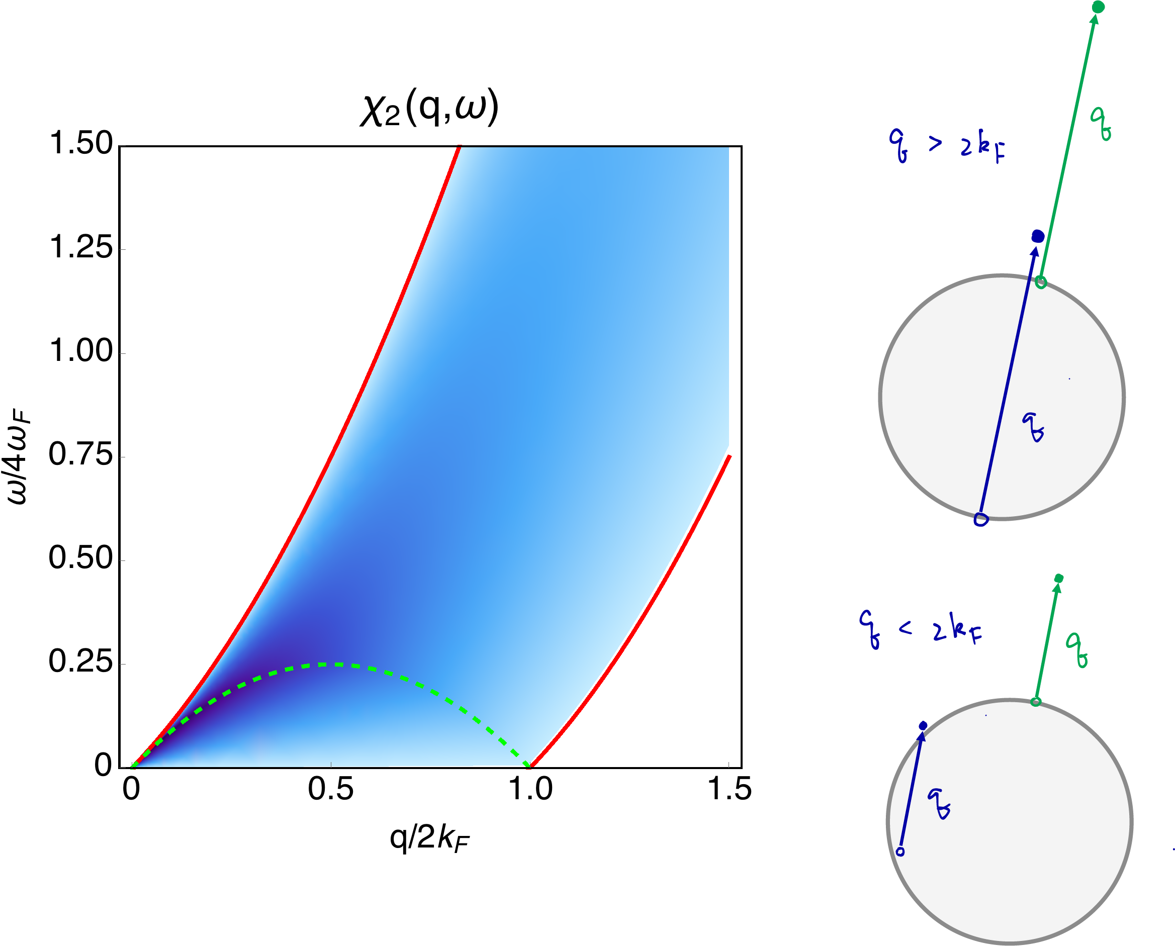
For the zero temperature spectral function, its imaginary part looks like
$\begin{matrix} (31) & Im χ_{s}^{0} (q, ω) = \frac{π}{ℏ} \int [d k] [θ (ω_{F s} - ω_{k + q s}) - θ (ω_{F s} - ω_{k s})] δ (ω - ω_{k + q s} + ω_{k s}) \end{matrix}$
$\boldsymbol k$ $\boldsymbol k+\boldsymbol q$ $\omega_{\boldsymbol k+\boldsymbol q} - \omega_\boldsymbol k=\omega$ $\boldsymbol k$ $\boldsymbol k+\boldsymbol q$ $\hbar\omega$ $\boldsymbol k+\boldsymbol q$ $\boldsymbol k$ $q$ $\omega$ plane in which the electron-hole pair generation through energy absorption is termed the particle-hole continuum.
$q$ $\omega \ge 0$ , as is graphically depicted in the figure above.
- $0<q<2k_F$ , the transition energy can be arbitrarily close to zero.
- $q>2k_F$ $\hbar^2[(q-k_F)^2-k_F^2]/2m$ .
- $q$ $\hbar^2 (k_F+q)^2/2m - \hbar^2 k_F^2/2m=\hbar^2(q^2+2k_Fq )/2m$ . These indeed yield the bounds of the particle-continuum, as in indicated by the red curves in panel on the left. This much can be easily established without explicitly writing down the spectral function, which can in fact be evaluated analytically for ground-state uniform electron gases.
Inspecting
$\begin{matrix} (32) & \begin{aligned} Im χ_{s}^{0} (q, ω) & = g (0) \frac{π}{8 x} [(1 - (\frac{u}{x} + x)^{2}) θ (1 - (\frac{u}{x} + x)^{2}) \\ - (1 - (\frac{u}{x} - x)^{2}) θ (1 - (\frac{u}{x} - x)^{2})] \\ with u = \frac{ω}{4 ω_{F s}} . \end{aligned} \end{matrix}$
$x<1$ $u/x-x <1$ $u/x+x<1$ $x$ $\eqref{eq:abc}$ $u$ $u=-x^2+x$ , indicated by the dashed green line.

Notes and references

1 Not true if there is interaction, in which case we only have

χ_{↑↓} = χ_{↓↑}

$\chi_{\uparrow \downarrow }=\chi_{ \downarrow \uparrow}$ . ↩