Lecture 9

Today

• Streda formula

• Nearly generate perturbation theory

• A review of the tight-binding method

Reading

• Lecture notes

• Girvin & Yang: 7.4, 7.5, 7.6

1. Streda formula

From the semiclassical equation of motion

We find

So in a system with non-zero Berry curvature, there is change in the Fermi volume under a magnetic field, as

is unchanged.

For an insulator, this leads to curious result. Consider a 2D system, threaded by a magnetic flux $\mathrm{\Phi }(t)$$\Phi(t)$ in an circular area $S$$S$

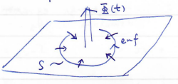
noting

is the charge transported across the boundary. We then find the Streda formula

We find for an insulator at $T=0$$T=0$

This is a curious result. That is, an insulator at $T=0$$T=0$ can also carry a nonzero anomalous current (it will be quantized!).

2. Nearly degenerate perturbation theory

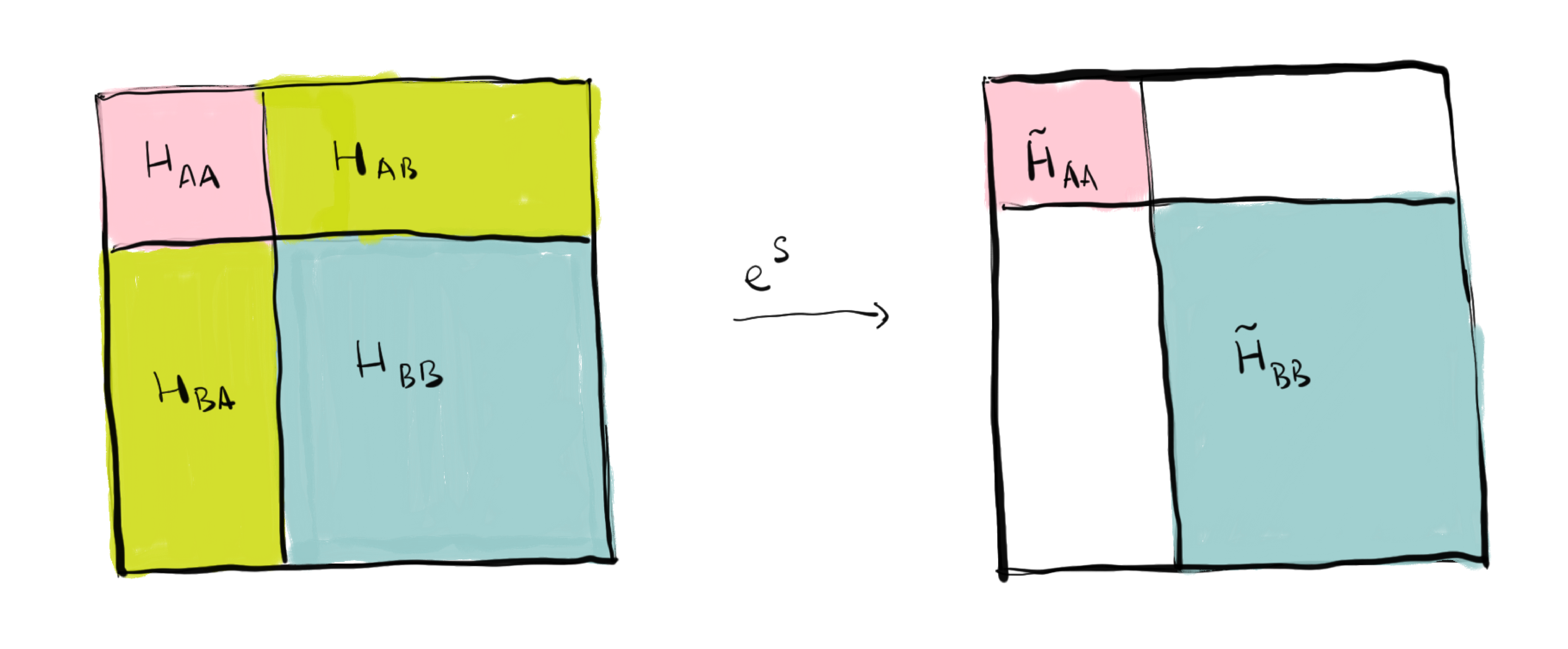
The degenerate perturbation theory (DPT) is a versatile tool for down-folding Hamiltonian into an effective Hamiltonian valid in a reduced Hilbert space. The DPT also goes by many different names in different contexts, such as the Löwdin perturbation, the Foldy–Wouthuysen transformation in relativistic quantum mechanics, or Fröhlich-Nakajima transformation in electron-phonon coupling, Schrieffer-Wolff transformation in the Kondo problem and quantum optics,¹ and so on.

The problem is formulated as follows. If we have a Hamiltonian of the form

where $H$$H$ is exactly solved, so we know all its eigenstates. $0\le \lambda \le 1$$0\le \lambda\le1$ sis a parameter controlling the strength of perturbation.

The typical scenario for the use of the DPT is as follows. The eigenstates of $H$$H$ has a low-energy subspace, separated from the other states by a finite energy gap $\mathrm{\Delta }$$\Delta$. Because the high-energy excitations make only small contribution to the system's physics, we would like a systematic approach for removing these unwanted degrees of freedom. The goal is to write an effective Hamiltonian only in low-energy subspace, within which the energy differences are smaller than $\mathrm{\Delta }$$\Delta$. Let's use $n,m$$n,m$ etc to label the states in the low-energy subspace, and $\alpha ,\beta$$\alpha,\beta$ other states.

The trick for doing this is performing a unitary transformation on the Hamiltonian

where $S$$S$ is an antihermtian operator, i.e. $S^{†}=-S$$S^\dagger =-S$, such that $e^{\lambda S}$$e^{\lambda S}$ is unitary.

We then expand $e^{\lambda S}$$e^{\lambda S}$ in a power series

Inserting this into Eq. $\text{(9)}$$\eqref{eq:unit}$, and collecting terms in ${\lambda }^p{\tilde{H}}^{(p)}$$\lambda^p\tilde H^{(p)}$, we find

For a second-order theory, we require that

which is an operator equation in $S^{(1)}$$S^{(1)}$. Solving for $S$$S$ we find

where $a,b$$a,b$ refer to any state, whether or not in any subspace.

Now the Hamiltonian to second order of perturbation is

When substituted back, this leads to

If the ground states are strictly degenerate $E_n=E_n^{\prime }=E_0$$E_n=E_n'=E_0$, we find

which is precisely Eq. (39.4) in Quantum Mechanics: Non-relativistic theory ( Landau and Lifshitz, Pergamon 1977). For a somewhat elementary and systematic discussion, you may find Zwiebach's notes useful, where the third order results are computed.

Now we have reduced our Hilbert space, at the price of complicating our Hamiltonian with $\tilde{H}$$\tilde H$. We often find this new Hamiltonian is still degenerate, so we need another round of elimination; in this fashion, we may go through several levels of description, and successive degeneracy breakings with smaller and smaller energy scales

3. Application: hopping band of a diatomic chain

Now for a monatomic chain, the tight-binding Hamiltonian (or hopping Hamiltonian) is

Note that we have not included spin in this Hamiltonian. We assume that electrons are spinless Fermions, following the Fermi-Dirac distribution², such that

When acting on the one-particle subspace, Eq. $\text{(17)}$$\eqref{eq:hop}$ is very easy to understand. goes much further, in that it also specifies the evolution of states with many particles. Consider $c_2^{†}{c}_1$$c_2^\dagger c_1$ on a chain: it annihilates a fermion on site 2 (or gives 0 if there is none), and creates one on site 1, i.e. it hops a fermion from 1 to 2. Note the economy of the second-quantized notation: this term encodes $2N-2$$2 N−2$ distinct matrix elements, from $|010\cdots 0⟩\to |100\cdots 0⟩$$|010\cdots 0\rangle → |100 \cdots 0\rangle$, all the way to $|011\cdots 1⟩\to |101\cdots 1⟩$$|011\cdots 1\rangle → |101 \cdots 1\rangle$. See Figure below. Locality means that each particle’s hopping is independent of the configuration of faraway particles, as common sense would suggest, and second-quantized notation is tailored to encode such behaviours succinctly

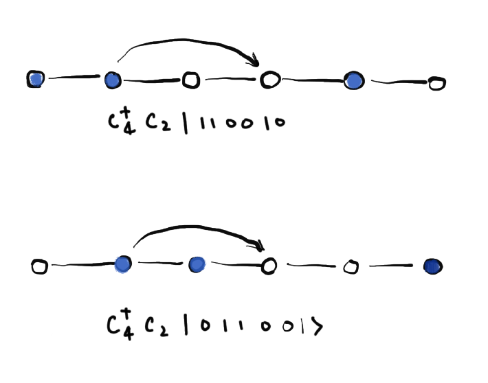
Figure 1: Compactness of the second-quantized form of the hopping term. The processes shown (and many more) have distinct matrix elements, but are described by the same operator $c^{†}(2)c(1)$$c ^\dagger (2)c(1)$.

For $H$$H$ to be Hermitian, we have $t(x,x^{\prime })=t(x^{\prime },x{)}^{\ast }$$t(x,x') =t(x',x)^*$ . Translation symmetry indicates that $t(x,x^{\prime })=t(x-x^{\prime })$$t(x,x')=t(x-x')$. The creation/annihilation operator formalism is handy because it is adapted to the locality of physical laws. If we had, say, a random Hamiltonian, with comparable matrix elements between any pair of states, this would look no simpler in second-quantized form: one might as well simply list all $2N\times 2N$$2 N ×2 N$ matrix elements. But real Hamiltonians are local: the amplitude to hop or interaction strength involves a finite number of nearby sites (or, at least, decays rapidly with distance) Thus a physical operator, which has many possible matrix elements, reduces to one or two terms in second quantized form.

In interacting systems, we get additional terms, which usually involve more than two operators. Usually the fermion number is conserved, so each term has the same number of creation and annihilation operators, but this rule is violated in the BCS mean-field Hamiltonian for superconductivity, which has terms have with two creations or two annihilations. But an ironclad rule is that the number must be even.

Now we consider the Fourier transform of the creation and annihilation operators

where $N$$N$ in the first equation is the number of unit cells in the macroscopic sample, and $N$$N$ in the second equation is the number of $k$$k$-points in the Brillouin zone.

The anticommutation relation in Eq. $\text{(18)}$$\eqref{eq:anticom}$ translates to

Inserting the expansion into Eq. $\text{(17)}$$\eqref{eq:hop}$, we find the diagonalized Hamiltonian

where the dispersion relation

is the Fourier transform of the hopping.

In the case of 1D chain with nearest-neighbor hopping only

then we have

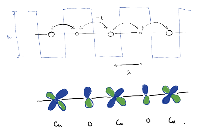
Now we consider a diatomic chain, created by making the on-site energies of consecutive atoms alternate. So the Hamiltonian reads

We find that the Hamiltonian in Fourier space is

where we have introduced a pseudospin

with

where $t_k=-t(1+e^{2\mathrm{i}ka})$$t_k = -t(1+e^{2\mathrm ika})$. Diagonalizing, we find that

But to grasp it, or to generalize it to a complex geometry, it is best to approach from the complementary limits of weak or strong potential. The $\mathrm{\Delta }\ll t$$\Delta\ll t$ limit is analogous to the nearly-free-electron (NFE) approximation to band structure.

The other limit, $\mathrm{\Delta }\gg t$$\Delta \gg t$, calls for off-diagonal second-order perturbation. Our zero-order Hamiltonian $H$$H$ is $V(x)$$V (x)$, which has many degenerate ground states of energy $-\mathrm{\Delta }/2$$−\Delta/2$, namely any of the even orbitals. The perturbation theory yields,

Then

where ${\epsilon }_{\text{well}}$$\varepsilon_{\text{well}}$ includes a small correction from diagonal second-order perturbation. You can check the result by comparing it with the exact result $\text{(29)}$$\eqref{eq:ediatomic}$ expanded in powers of $t/\mathrm{\Delta }$$t/\Delta$.

Also shown in the figure a one-dimensional cartoon of the alternating copper d orbitals and oxygen p orbitals found in the CuO2 plane of a high-temperature superconductor. In the customary treatment of that system, the oxygen $p$$p$ orbitals are eliminated in favor of the copper $d$$d$ orbitals.

References and notes