Lecture 10
03/23/2023, Th.
Today
Examples of TB models
Boltzmann equation
Semiclassical transport theory
Reading
Girvin & Yang ch. 8
1. Further examples of tight-binding models
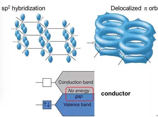
1.1 Graphene
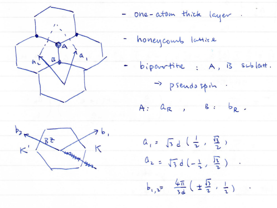
The corner of the Brillouin zone:
There are only two distinct corners, the others are related to
The Hamiltonian involving nearest neighbor hopping of
where
Substituting in the Fourier expansion, we find
where
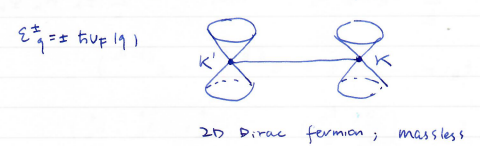
The dispersion relation is simply
At
Conduction and valence bands touch at
So the Hamiltonian matrix near
Near
So we would write
where
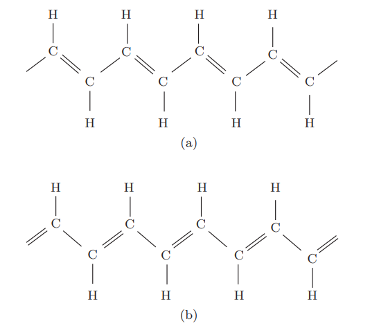
1.2 Polyacetylene and the SSH model
The 1D atomic chain also features a Dirac point at the Brillouin zone boundary. Two ways to lift the degeneracy:
staggered lattice potential: we have discussed.
staggered hopping: Su-Schrieffer-Heeger (SSH) model
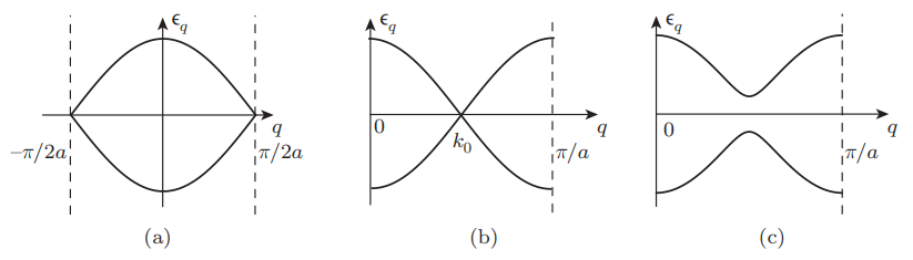
Expanding near
At half-filling (半满), the change of energy from the distortion is
The corresponding lattice energy increase is
where
So we find
So for sufficiently small distortion, this quantity goes negative. The implication is that the linear monatomic chain with half-filled electron band is always unstable against pairing distortion. This is the Peierl's instability.
2. The Boltzmann equation
The Boltzmann equation
where
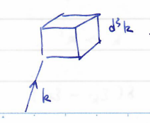
Consider the change of particle number in a phase space volume element
So
Local representative volume in which local equilibrium can be assumed
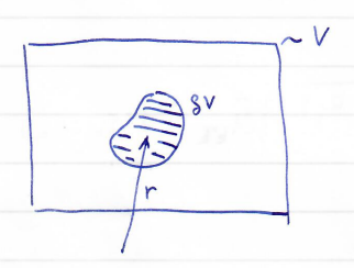
Locally, the equilibrium is referenced to local temperature, potential
3. The collision integral
We demonstrate the idea by considering the impurity scattering.
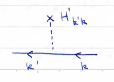
The scattering rate from
we take an impurity potential of the form
Some calculations
here
The above refers to a single electron. No information about the distribution is used.
Electrons with a distribution
The rate of change of
at Further simplification for isotropic system:
In Girvin and Yang's Eq. (8.108), the angular dependence of
Think about the first-order change in the distribution of
WLOG,
where
If you take
Now we have the relaxation-time approximation
The linearized Boltzmann equation
Approximations involved
-- isotropic, elastic scattering,
advantage: simple enough to get picture and results.
Example: Steady state:
Take
So the linear response theory is
Isotropic case, the longitudinal conductivity
This is recovers the Drude's law, with a little subtlety. In the Drude's law, the relaxation time should be
The anomalous Hall effect