Lecture 12
03/30/2023, Th.
Today
Landauer formula
1D localization
Reading
Girvin & Yang ch. 10.2-10.4
1. Beyond Boltzmann: quantum effects
Shubnikov-de Haas:
Cyclotron resonance
Localizaiton: weak, strong and many-body
insulator: Einstein relation
Band insulator
Mott insulator
Anderson insulator: MIT by Anderson transition is a quantum phenomenon
Plan
Landauer formula (leads to 1d localization, and later QHE edges)
Diffusion, and weak localization
Anderson localization
2. Landauer formula
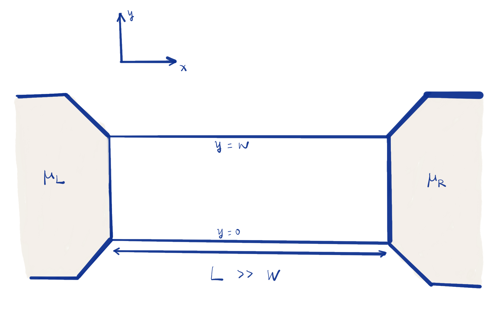
We consider a device made of a 2-dimensional electron gas (2DEG), confined in a
where
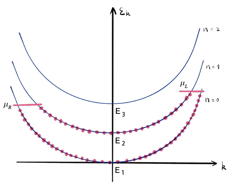
The electron states in a confined electron gas
where
We also impose a voltage by having different chemical potentials, say
in the two leads, so the voltage is given in the relation
Electrons entering the wire from the left electrode are right-moving with chemical potential
Electrons entering the wire from the right electrode are left-moving with chemical potential
We now compute the current
The above integral is
zero if
So if we introduce the conductance
then each open channel contributes a
where the number of open channels is
We introduce the quantum unit of conductance

The derivation above is independent of the details of the band structure. So, so long as the wire is perfect, the conductance is determined by the number of open channels, without regard to the shape of the bands.
The paradox: a perfect wire has finite conductance, and therefore finite resistance. This means there must be dissipation.
So where does the dissipation happen? It happens in the leads (or reservoirs), so that the electrons entering /exiting the wire assume chemical potentials
The electron from the left reservoir must dissipate energy in the right reservoir;
The device resistance (i.e. global) of the ideal wire is really the contact resistance.
Now we turn to an imperfect wire. Suppose there is one scatterer in the wire.
For the nth band, suppose the reflection amplitude (反射几率幅) is
ignore band hopping, for the moment.
Then
Again, the integrand (被积函数) is zero, unless
where
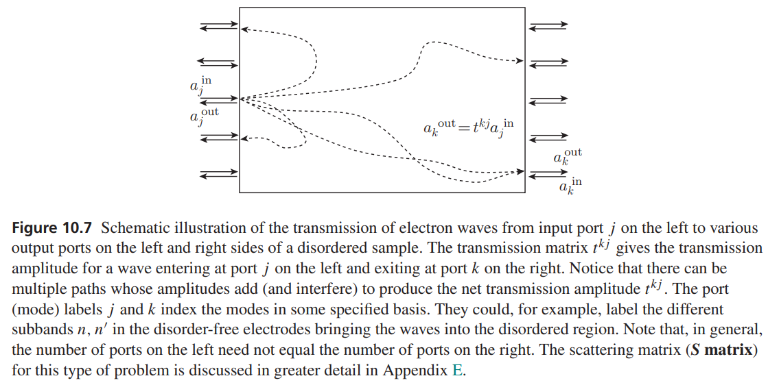
More generally, when there is band hopping. An electron enters the wire at
3. Multiterminal device
M. Büttiker generalized the Landauer formula, to multi-terminal device. Shown below is four-terminal device (or a
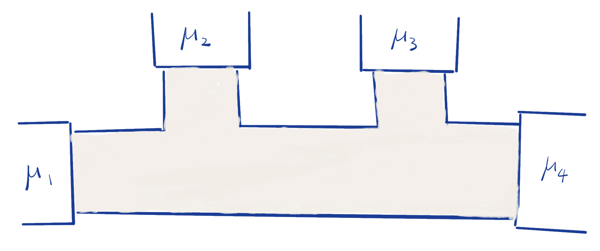
Then by the Landauer formula the net current entering terminal
where
Suppose all reservoirs have the same chemical potentials, then all currents vanish. We have sum rule (求和规则)
Then
If a terminal has no net current in or out, it is called a voltage probe. To make a voltage probe, we need
Now for the four-terminal device, if we float terminals 2 and 3, and there is a current flowing between terminal 1 and 4, this is the so-called four-terminal measurement. Then the voltage between 2 and 3 is
Importantly, if there are no scatterers in the region between ports 2 and 3 and if the ports are perfectly left/right symmetric, one can show that
More generally speaking, adding contacts to the system, even in the form of voltage probes (which supposedly do not affect the circuit classically), inevitably changes the system and results of measurements involving other contacts. This is yet another example of the fact that in a quantum world any measurement inevitably affects the objects being measured.
4. Two scatterers
Suppose there are two scatterers in a two-terminal device.
like Fabry-Perot cavity
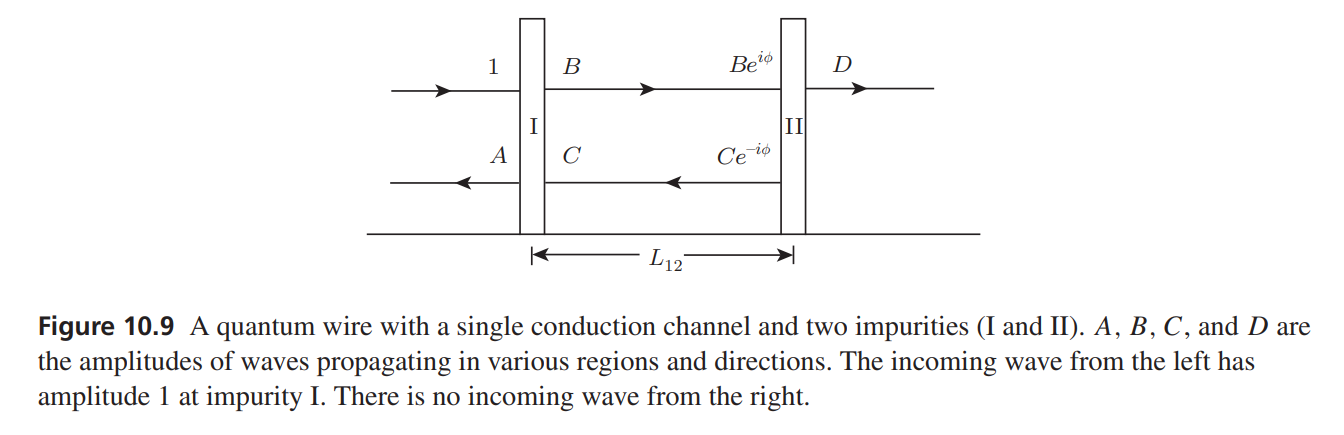
Let's do the accounting
where where the primed variables are the transmission and reflection amplitudes for right incidence (which have the same magnitude as their left-incidence counterparts but possibly different phases). The phase picked up by the traveling wave is
Solving, we find
The conductivity depends on
This huge change depending on the separation between scatterers is a result of interference of waves from multiple reflection in the cavity.
Thus
To better understand the interference phenomenon, let us consider the dimensionless resistance
This definition comes form the following considerations. We have said
For the two-impurity case
We find
Quantum resistances connected in series (串联) do not add up!
The average resistance,
on average, the resistance of two impurities is bigger than the sum of the resistances of individual impurities!
5. Many scatterers:1D localization
Landauer 1970: a sequence of nearly transparent (透明) scatterers,
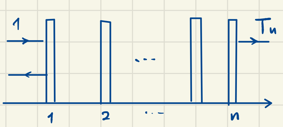
the increment is bigger than
which points squarely to localization as the wire length increases.
There is a bug in the above analysis:
the distribution of
We need something that is
Anderson (1980): log
If the two scatterers are identical
So
Therefore
where
This is the 1D localization. That is, waves cannot propagate in a 1D media with random disorder, due to interreference from multiple reflections. It can also be rigorously proved, in the case of electrons in 1D. Mott and Twose (1961) showed that all eigenstates of 1D electron system get localized with disorder (at low temperatures of course in order for the quantum interference effects to be significant).