Lecture 13
04/03/2023, M.
Today
Anderson model
Wave propagation (conduction) as diffusion
Quantum correction
1. Anderson's model (1958)
Anderson's model describes an electron in a 1D lattice with random potential
where is the random variable
If
In a "locator expansion", Anderson find that there exists a critical
Following Anderson's model, Mott (莫特) developed the idea of mobility edge for intermediate disorder, as shown in the figure below. With disorder, a band can be divided into delocalized (extended) and localized ranges, joined at energies called the “mobility edges”. Mott had an argument (not rigorous) that extended and localized states cannot exist at the same energy. When
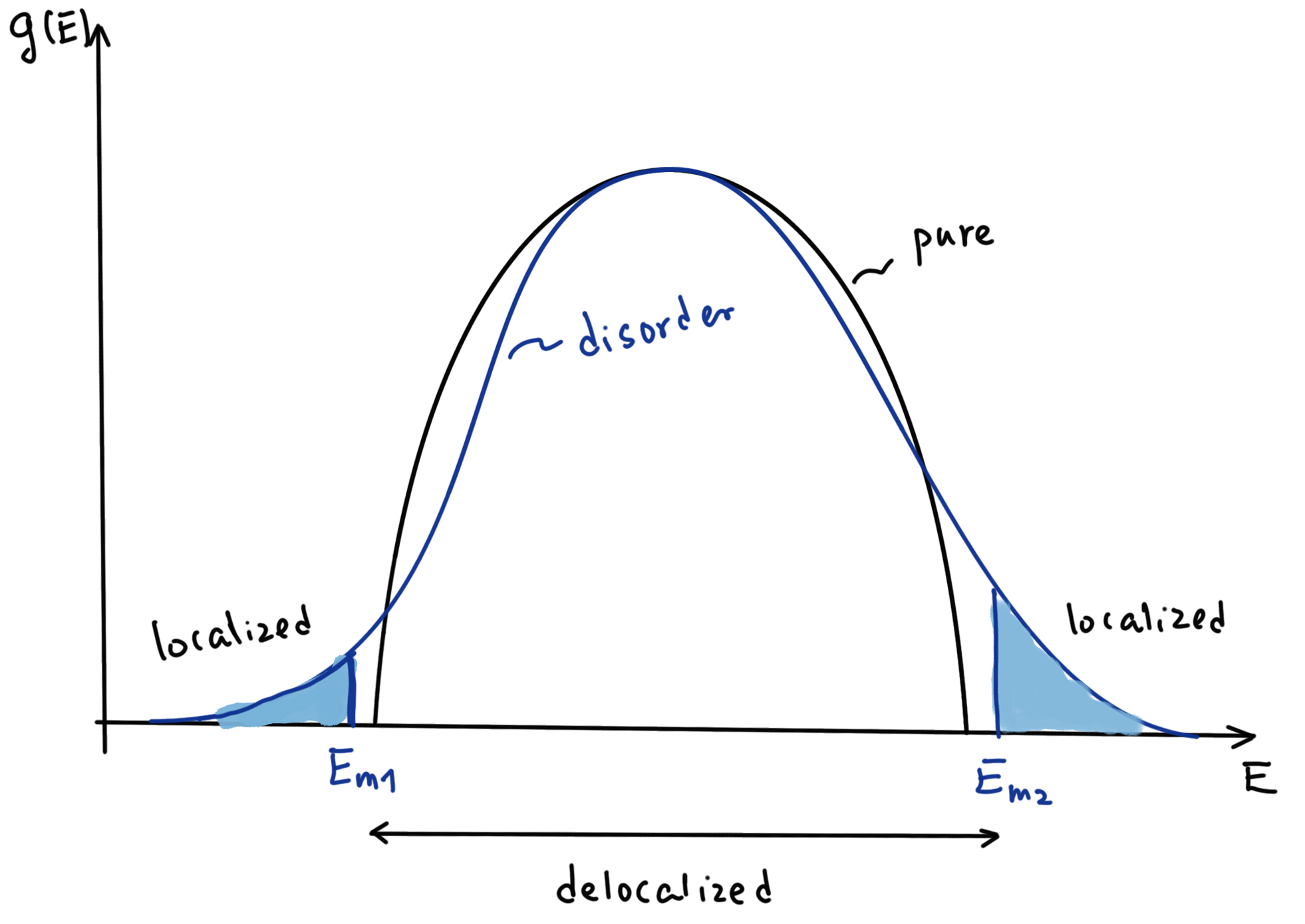
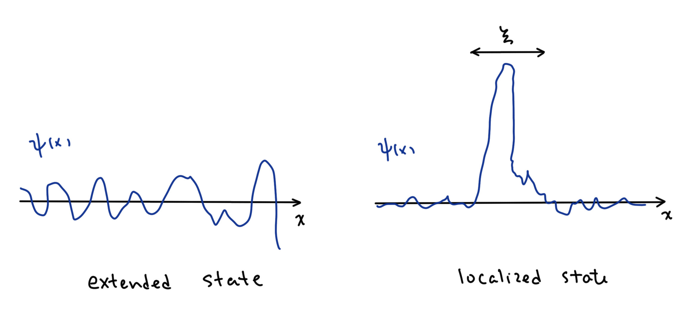
How do we quantify localization? We can eyeball the wavefuncitons. The localized state has a localized wavefunction, which has most of its weight in a finite length scale, called the localization length
In actual calculations, you can use the inverse participation ratio
If
extended state:
localized:
2. Classical diffusion
Fick's law
with equation of continuity
leads to Fick's second law
Fourier transform
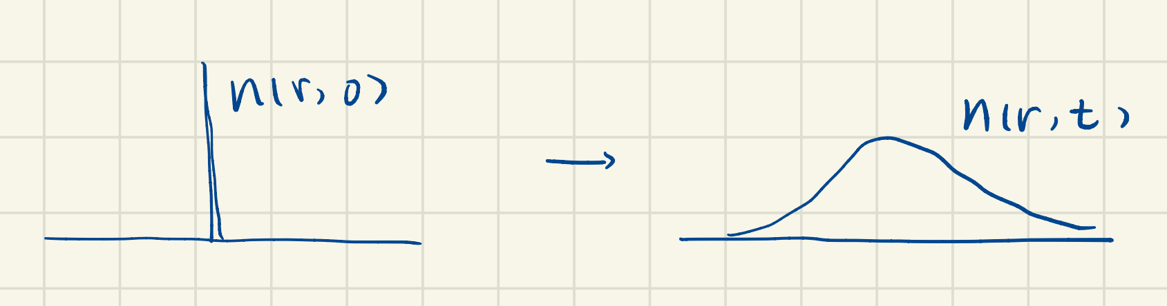
Relating to random walks. The central limit theorem tells us that the sum of a large number of random variables is Gaussian distributed and has a variance (width squared) proportional to the number of steps. This gives the probability density
where
Comparing to the diffusion equation, we have:
Also introduce the diffusion length
Since only the electron at the Fermi energy contributes to conduction, we can assume the electrons are moving at a speed
The number of steps in time t is
where
The mean square step length
So we find
we have
Substitute into the Einstein relation
So, we have developed a physical picture that connects the evolution of quantum wave functions with the classical notion of diffusion, which in turn can be viewed as random walks form scatterer to scatter in the sample.
3. Multiple scattering as diffusion
path integral:
where the semiclassical is introduced, by summing only over the classical paths. A classical path is one which minimizes the action
So probability density is
Disorder averaging:
where
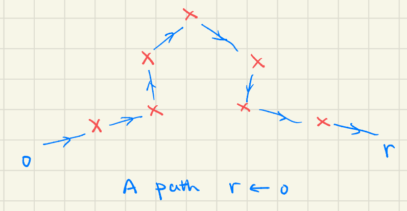
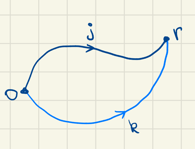
Since an electron starting at (0,0), can take any classical path to reach (r,t), with equal probability, we expect
So a semiclassical propagation of quantum waves in a random medium can be described as diffusion.
4. Quantum correction
Consider a self-intersecting path,
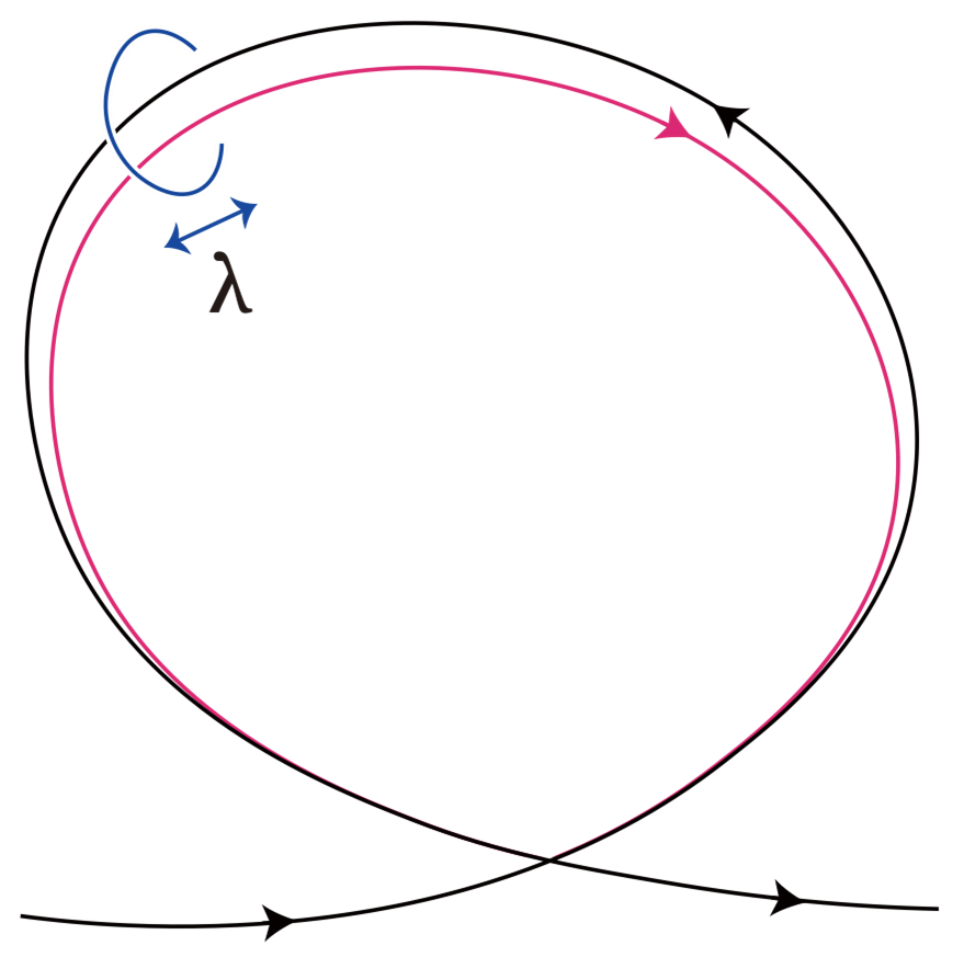
Time-reversal symmetry means the action does not change under time reversal
so
The probability of return is
Since by our construction,
This is the picture of electron localization via quantum interference: increased probability of return.
Let's now formulate this in k-space, in terms of elastic scattering of electrons at on the Fermi surface, from
where
Backscattering:
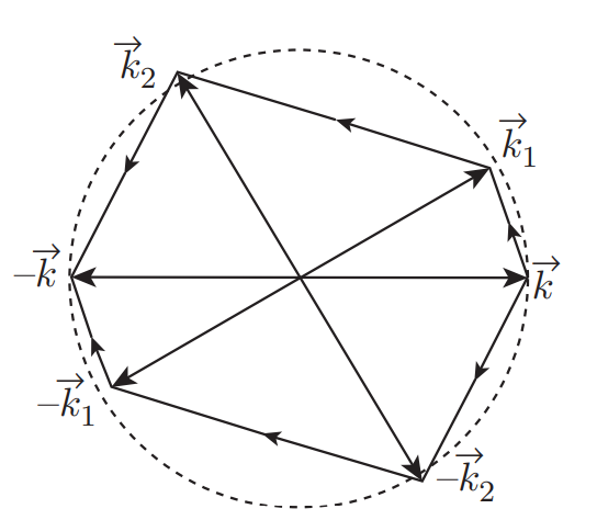
for the time-reversed path
Time reversal symmetry means:
So in the k-space, the amplitudes of backscattering via time-reversed paths are the same. Therefore, they will survive disorder averaging.
To sum up, the quantum correction to semiclassical diffusion
real space: increased probability of return
k-space: enhanced back scattering