Lecture 15
04/10/23, M.
Next: Berry phase and topology of Bloch bands
Ch. 13, 12, 14 of G&Y.
1. Geometry and topology
Instead of offering a systematic survey of concepts of topology, I offer an appetizer by with the Gauss-Bonnett theorem
The Gauss–Bonnet theorem provides a quantitative relation between the curvature (a local quantity) and its topology (a global property) of a surface.
where
Take a sphere of radius
Then
consequently,
The topological aspect of this is that the integral does not change if we continuously deform the sphere into a surface, the integral does not change. That is
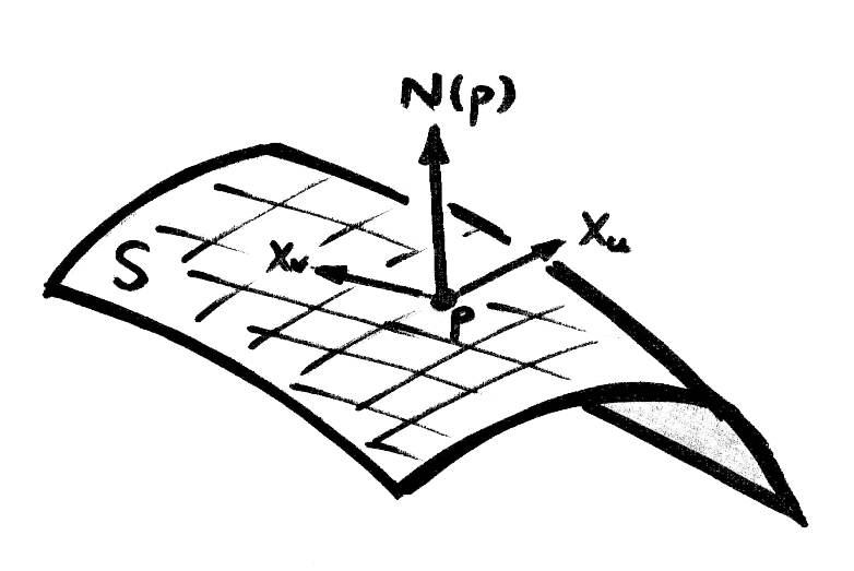
Consider a surface in
This is called the Gauss map, which maps a surface on to a unit sphere. The Gaussian curvature is
So
So Gaussian curvature is like the Jacobian of the Gauss map.
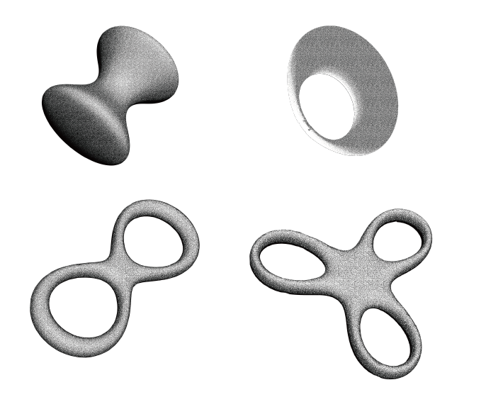
Further example: torus
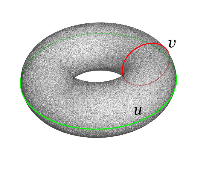
with
At a point
We find the Gaussian curvature to be
The surface element is
We then find the total curvature to be zero. So
Quantization: If the surface is closed, one expects its image under the Gauss map to wrap around the sphere integer number of times. Then the value of
Global: while curvature is local,
Invariant: because
New physics:
quantized property, robust against perturbation, and interaction
phase change: no symmetry change
Our goal: topology of Bloch bands
2. Geometric phase
We consider the adiabatic evolution of a semiclassical system.
The instantaneous eigen states
with the initial condition at
Adiabatic limit (绝热极限):
The Schrodinger equation
Inserting the adiabatic wavefunction into it, we find
where
Integrating, we find the geometric phase (几何相位)
The phase
U(1) gauge transformation
This means that
3. Berry phase
Now we inspect the geometric phase over a loop
where we have used the Stoke's theorem in the second line. The quantity
Example: 2D Dirac fermion in graphene. Take one of the valleys
with the dispersion relations
For the Berry connection
So the Berry phase for an electron to revolve around the Fermi surface
It picks up a
This has very important consequences for transport in graphene. Instead of displaying enhancement of backscattering, there is a suppression of backscattering.
But there is a problem. The Berry curvature
so
How is this compatible with the Stokes' theorem? The answer is: there is singularity.