Lecture 16

04/13/2023, Th.

Today

Berry connection and curvature
Examples: A-B phase, two-level system
Bloch bands

$\Omega_{ab}$

We use the fact

\begin{matrix} (1) & \begin{matrix} \frac{\partial}{\partial λ_{a}} ⟨ n^{'} | H | n ⟩ = δ_{n n^{'}} \frac{\partial E_{n}}{\partial λ_{a}} \\ = ⟨ \partial_{a} n^{'} | n ⟩ E_{n} + E_{n^{'}} ⟨ n^{'} | \partial_{a} n ⟩ + ⟨ n^{'} | \frac{\partial H}{\partial λ_{a}} | n ⟩ \end{matrix} \end{matrix}

$n'\neq n$ ,

\begin{matrix} (2) & ⟨ n^{'} | \frac{\partial H}{\partial λ_{a}} | n ⟩ = (E_{n} - E_{n^{'}}) ⟨ n^{'} | \partial_{a} | n ⟩ \end{matrix}

Then

\begin{matrix} (3) & \begin{matrix} Ω_{a b} = \frac{\partial A_{b}}{\partial λ_{a}} - \frac{\partial A_{a}}{\partial λ_{b}} \\ = i [⟨ \partial_{a} n | \partial_{b} n ⟩ - ⟨ \partial_{b} n | \partial_{a} n ⟩] \\ = i \sum_{n^{'} \neq n} [⟨ \partial_{a} n | n^{'} ⟩ ⟨ n^{'} | \partial_{b} n ⟩ - ⟨ \partial_{b} n | n^{'} ⟩ ⟨ n^{'} | \partial_{a} n ⟩] \end{matrix} \end{matrix}

Finally we have

\begin{matrix} (4) & Ω_{a b} = i \sum_{n^{'} \neq n} \frac{⟨ n | \partial_{a} H | n^{'} ⟩ ⟨ n^{'} | \partial_{b} H | n ⟩ - (a \leftrightarrow b)}{(E_{n} - E_{n^{'}})^{2}} \end{matrix}

2. A-B phase a Berry phase

$B=0$ $\boldsymbol a(\boldsymbol r)$ is not.

This can be derived heuristically in a semiclassical approximation of the path integral, which says the transition is characterized by the phase of the classical path. The amplitude is

\begin{matrix} (5) & e^{i S [Γ] / ℏ} \end{matrix}

$S$ is the action. With the magnetic field or vector potential

\begin{matrix} (6) & S = \int_{0}^{t} d t^{'} L (\dot{r}, r) \end{matrix}

with

\begin{matrix} (7) & L = L_{0} - e a \cdot \dot{r} . \end{matrix}

So there is a magnetic change of phase

\begin{matrix} (8) & Δ ϕ = - \frac{e}{ℏ} \int_{Γ} d r \cdot a (r) \end{matrix}

$\Gamma$ $\Gamma'$ . The phase difference between these two events are then given by

\begin{matrix} (9) & - \frac{e}{ℏ} (\int_{Γ} + \int_{- Γ^{'}}) a \cdot d r = - \frac{e}{ℏ} Φ = - 2 π \frac{Φ}{Φ_{0}} \end{matrix}

$\Phi$ is gauge invariant (规范不变的)

We now illustrate how this phase can be formulated in terms of a Berry phase. We suppose the charged particle is an electron confined in a box (a confining potential), and is moved along with the box around the magnetic flux.

\begin{matrix} (10) & H = \frac{1}{2 m} (p + e a)^{2} + \underset{confining potential}{\underset{⏟}{V (r - R)}} \end{matrix}

$a=0$ $R$ $|\psi_0(R)\rangle$ .

$B$ $B=0$ . The presence of the vector potential amounts to a gauge transformation

\begin{matrix} (11) & | ψ (R) ⟩ = \exp (- \frac{i e}{ℏ} \int_{R}^{r} a (r^{'}) \cdot d r^{'}) | ψ_{0} (R) ⟩ \end{matrix}

$\nabla\times a =0$ inside the box, the line integral is path independent so along as it is in the box.

\begin{matrix} (12) & \begin{aligned} H | ψ (R) ⟩ & = \exp [- \frac{i e}{ℏ} \int_{R}^{r} a (r^{'}) d r^{'}] (\frac{p^{2}}{2 m} + V (r - R)) | ψ_{0} (R) ⟩ \\ = \exp [- \frac{i e}{ℏ} \int_{R}^{r} a (r^{'}) d r^{'}] E | ψ_{0} (R) ⟩ \\ = E | ψ (R) ⟩ \end{aligned} \end{matrix}

The Berry connection

\begin{matrix} (13) & ⟨ ψ (R) | i \frac{\partial}{\partial R} | ψ (R) ⟩ = ⟨ ψ_{0} (R) | i \frac{\partial}{\partial R} | ψ_{0} (R) ⟩ - \frac{e}{ℏ} a (R) \end{matrix}

The Berry phase

\begin{matrix} (14) & γ = - \frac{e}{ℏ} \oint_{C} a \cdot d R + i \int_{Σ} \underset{= 0 because ψ_{0} (r - R) is real.}{\underset{⏟}{(⟨ \frac{\partial ψ_{0}}{\partial R^{α}} ∣ \frac{\partial ψ_{0}}{\partial R^{β}} ⟩ - α \leftrightarrow β)}} d σ \end{matrix}

Then we see that A-B phase is just the Berry phase.

3. Two-level system

The Hamiltonian of a two-level system can be written as

\begin{matrix} (15) & \begin{matrix} H = h \cdot σ = h_{x} σ_{x} + h_{y} σ_{y} + h_{z} σ_{z} \\ = [\begin{matrix} h_{z} & h_{x} - i h_{y} \\ h_{x} + i h_{y} & - h_{z} \end{matrix}] \end{matrix} \end{matrix}

$\boldsymbol h$ in spherical coordinates

\begin{matrix} (16) & h = (h_{x}, h_{y}, h_{z}) = h (\sin θ \cos ϕ, \sin θ \sin ϕ, \cos θ), h > 0. \end{matrix}

$\varepsilon_\pm=\pm h$ . Let's focus on the lower branch

\begin{matrix} (17) & \begin{matrix} | ψ_{-} ⟩ = [\begin{matrix} e^{- i ϕ} \sin \frac{θ}{2} \\ - \cos \frac{θ}{2} \end{matrix}] \end{matrix} \end{matrix}

Let's compute the Berry connection

\begin{matrix} (18) & \begin{aligned} A_{θ} = ⟨ ψ_{-} | i \frac{\partial}{\partial θ} | ψ_{-} ⟩ = 0 \\ A_{ϕ} = ⟨ ψ_{-} | i \frac{\partial}{\partial ϕ} | ψ_{-} ⟩ = \sin^{2} \frac{θ}{2} \end{aligned} \end{matrix}

So the Berry curvature is

\begin{matrix} (19) & Ω_{θ ϕ} = \frac{1}{2} \sin θ . \end{matrix}

$h$ $(\theta,\phi)$ $\partial \Sigma$ , then the Berry phase is

\begin{matrix} (20) & \begin{matrix} γ = \int_{Σ} d θ d ϕ Ω_{θ ϕ} = \frac{1}{2} \int_{Σ} \sin θ d θ d ϕ \\ = \frac{1}{2} \times solid angle subtended by Σ . \end{matrix} \end{matrix}

$\Sigma$ $\gamma=2\pi$ . On the other hand

\begin{matrix} (21) & γ = \oint_{\partial Σ} A \cdot d l = 0 \end{matrix}

$\partial \Sigma =\emptyset$ . This is apparently in contradiction with the Stokes theorem.

$A_\theta, A_\phi$ $A_\phi(\pi) = 1$ $h$ value. This kind of singularity is called the Dirac string.

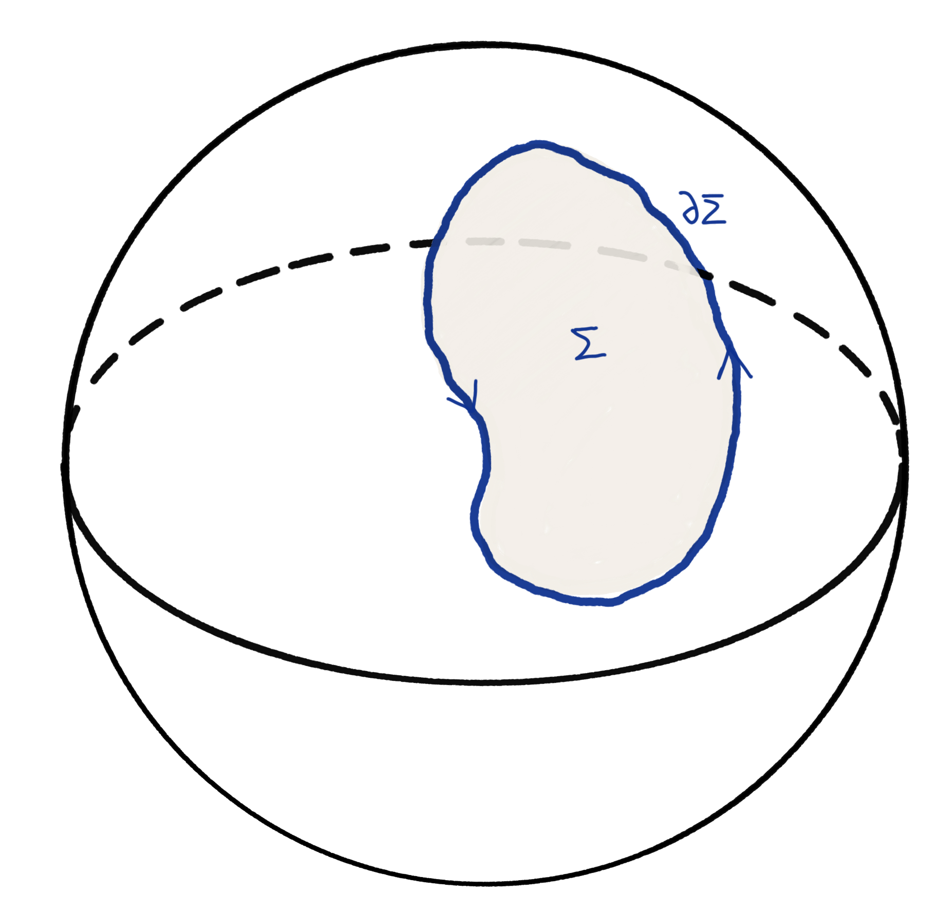
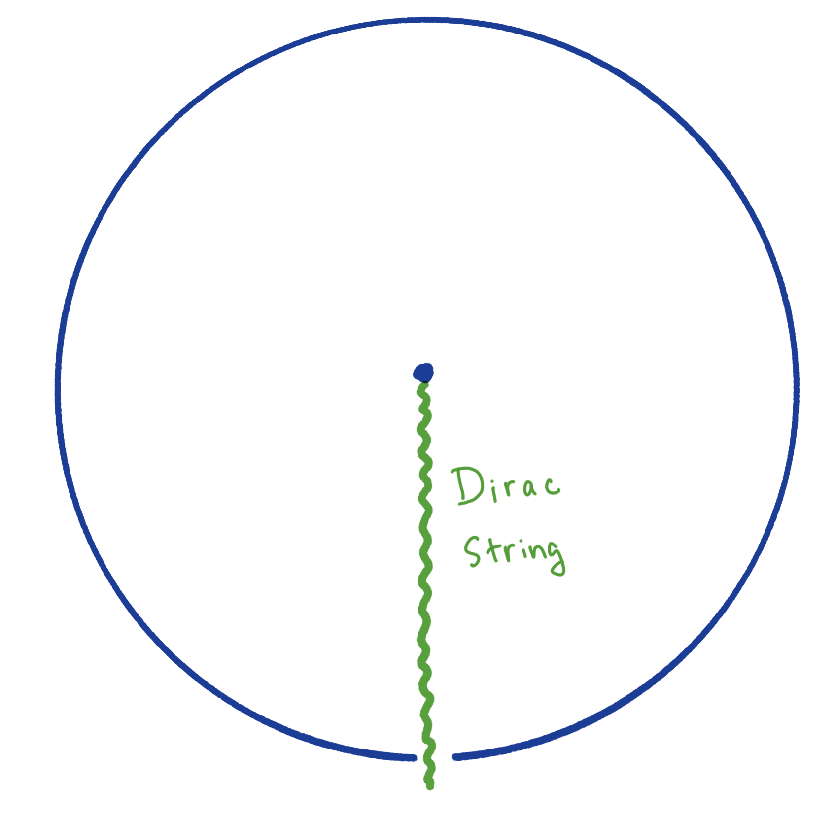
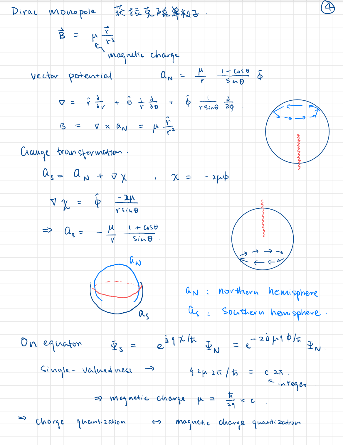
This is analogous to the Dirac's magnetic monopole, if we switch to the Cartesian coordinates

\begin{matrix} (22) & Ω_{a b} = Ω_{θ ϕ} \frac{\partial (θ, ϕ)}{\partial (h_{a}, h_{b})} = \frac{1}{2} \frac{\partial (ϕ, \cos θ)}{\partial (h_{a}, h_{b})} \end{matrix}

we find

\begin{matrix} (23) & \vec{Ω} = \frac{\vec{h}}{2 h^{3}} \end{matrix}

which is singular at the origin.

4. Geometric properties of Bloch bands

For a single electron in a periodic potential, Bloch theorem says its eigenstates are irreducible representation of lattice translation

\begin{matrix} (24) & H | ψ_{n k} ⟩ = ε_{n k} | ψ_{n k} ⟩ \end{matrix}

where the Bloch function has the following property

\begin{matrix} (25) & \begin{matrix} ψ_{n k} (r + R) = e^{i k \cdot R} ψ_{n k} (r) \\ ψ_{n k} (r) = e^{i k \cdot r} u_{n k} (r) . \end{matrix} \end{matrix}

$|u_{nk}\rangle$ $|\psi_{nk}\rangle$ .

We can now make the following transformation

\begin{matrix} (26) & H_{k} = e^{- i k \cdot r} H e^{i k \cdot r} \end{matrix}

which we will call the Bloch Hamiltonian. Then we have the following Schrodinger equation

\begin{matrix} (27) & H_{k} | u_{n k} ⟩ = ε_{n k} | u_{n k} ⟩ . \end{matrix}

We then define the Berry connection (again) of Bloch bands

\begin{matrix} (28) & A_{m n} (k) = ⟨ u_{m k} | i \partial_{k} | u_{n k} ⟩ \end{matrix}

$|u_{mk}\rangle$ are unit-cell normalized, so the above bra-ket signifies integral within one unit cell.

For this course, we will focus on usually problems involving a single band. The one-band (Abelian) Berry connection is

\begin{matrix} (29) & A_{n} (k) = ⟨ u_{m k} | i \partial_{k} | u_{n k} ⟩ \end{matrix}

with which we can introduce the Berry curvature (again, Abelian)

\begin{matrix} (30) & Ω_{n} (k) = \nabla_{k} \times A_{n} (k) \end{matrix}

Let's now place the system in a uniform electric field

\begin{matrix} (31) & E = - \dot{a} \end{matrix}

The crystal Hamiltonian is

\begin{matrix} (32) & H = \frac{(p + e a)^{2}}{2 m} + V \end{matrix}

And the Bloch Hamiltonian

\begin{matrix} (33) & H_{k} = \frac{(p + e a + ℏ k)^{2}}{2 m} + V (r) \end{matrix}

but we may just define a new wavevector that depends on time

\begin{matrix} (34) & q (t) = k + \frac{e}{ℏ} a \end{matrix}

$q$ vectors

\begin{matrix} (35) & H_{q (t)} | u_{n q (t)} ⟩ = ε_{n q (t)} | u_{n q (t)} ⟩ . \end{matrix}

\begin{matrix} (36) & \dot{q} = - \frac{e}{ℏ} E \end{matrix}

Now consider the first-order wavefunction

\begin{matrix} (37) & | u_{n k}^{(1)} ⟩ = | u_{n k} ⟩ - i ℏ \sum_{n^{'} \neq n} \frac{| u_{n^{'} k} ⟩ ⟨ u_{n^{'} k} | \partial_{t} | u_{n k} ⟩}{ε_{n k} - ε_{n^{'} k}} \end{matrix}

The velocity operator

\begin{matrix} (38) & {\dot{r}}_{k} = \frac{i}{ℏ} [H_{k}, r] = \frac{\partial H_{k}}{ℏ \partial k} \end{matrix}

So the velocity to the first order of perturbation

\begin{matrix} (39) & v_{n k} = v_{n k}^{(0)} - i ℏ \sum_{n^{'} \neq n} \frac{⟨ u_{n k} | {\dot{r}}_{k} | u_{n^{'} k} ⟩ ⟨ u_{n^{'} k} | \partial_{t} | u_{n k} ⟩ - c.c.}{ε_{n k} - ε_{n^{'} k}} \end{matrix}

where the first term is the group velocity of the nth Bloch band, and the second term is the anomalous velocity (we will see how it reduces to the anomalous velocity in the anomalous Hall effect shortly).

$n\neq n'$

\begin{matrix} (40) & 0 = \partial_{k} ⟨ u_{n} | H_{k} | u_{n^{'}} ⟩ = (ε_{n^{'}} - ε_{n}) ⟨ \partial_{k} u_{n} | u_{n^{'}} ⟩ + ⟨ u_{n} | \partial_{k} H_{k} | u_{n^{'}} ⟩ \end{matrix}

we find that

\begin{matrix} (41) & \begin{matrix} v_{n k} = v_{n k}^{(0)} - \sum_{n^{'} \neq n} ⟨ \partial_{k} u_{n k} | u_{n^{'} k} ⟩ ⟨ u_{n^{'} k} | i \partial_{t} | u_{n k} ⟩ - c.c. \\ = v_{n k}^{(0)} - i (⟨ \frac{\partial u_{n k}}{\partial k} | \frac{\partial u_{n k}}{\partial t} ⟩ - c.c.) \end{matrix} \end{matrix}

So we have

\begin{matrix} (42) & v_{n k}^{a} = v_{n k}^{(0) a} - Ω_{k_{a} t} \end{matrix}

$-\Omega_{k_at}$ $a$ direction

\begin{matrix} (43) & Ω_{k_{a} t} = i (⟨ \frac{\partial u_{n k}}{\partial k_{a}} | \frac{\partial u_{n k}}{\partial t} ⟩ - ⟨ \frac{\partial u_{n k}}{\partial t} | \frac{\partial u_{n k}}{\partial k_{a}} ⟩) \end{matrix}

$\dot q$ $q$ $k$

\begin{matrix} (44) & \begin{matrix} v_{n k}^{a} = v_{n k}^{(0) a} - Ω_{k_{a} k_{b}} {\dot{k}}_{b} \\ = v_{n k}^{(0) a} - (\dot{k} \times \vec{Ω})^{a} \end{matrix} \end{matrix}

which is the same as what we have obtained from semiclassical dynamics.

Lecture 16

1. Multiband expansion for Ωab\Omega_{ab}

2. A-B phase a Berry phase

3. Two-level system

4. Geometric properties of Bloch bands

$\Omega_{ab}$