Lecture 17

04/19/2023, Th.

Today:

1. Anomalous velocity

So we have

(1)vnka=vnk(0)aΩkat

where Ωkat is the anomalous velocity in a direction

(2)Ωkat=i(unkka|unktunkt|unkka)

So combining with the expression for q˙ in electric field, and writing now q as k

(3)vnka=vnk(0)aΩkakbk˙b=vnk(0)a(k˙×Ω)a

which is the same as what we have obtained from semiclassical dynamics.

Note that (1) is somewhat more fundamental than (3), in the sense that (1) works even for 1D system whereas the latter only applies to 2D or 3D systems. We will look at a 1D example right away.

2. Adiabatic pumping in a 1D insulator

For an insulator at T=0, Boltzmann transport theory tells us there can be no current, even under external fields.

Let's consider the adiabatic current, arising from the anomalous velocity of one fully occupied band (insulator)

(4)j=eBZdk2πΩkt

in a cyclic process

(5)H(t+T)=H(t).

Then the number of electrons transported across the system in one time period is

(6) No. e transported c=0TdtBZdk2πΩkt

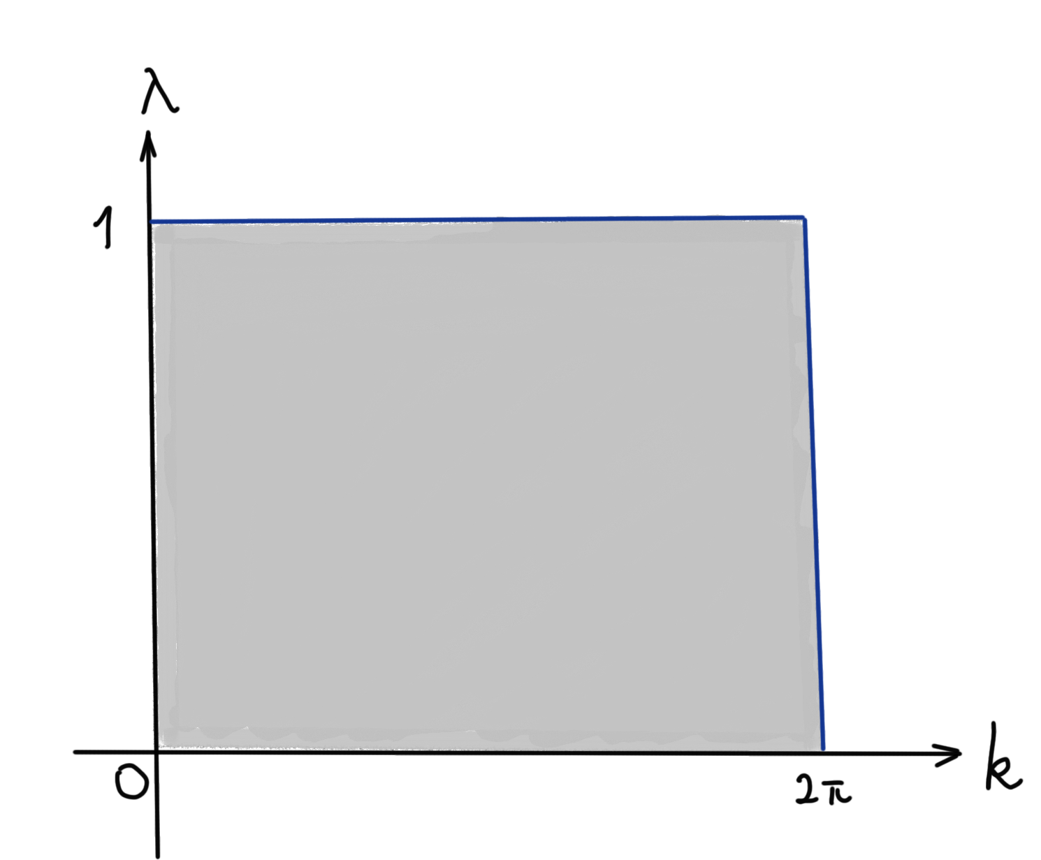
The region of integration is a rectangle

(7)[0,T]×[0,2π]

The integrand is periodic in the t-direction and in the k direction, because the Bloch functions at k and k+2π are the same physical state, so the Berry flux must be the same. This is like the region of integration is rolled up in k direction, and then in t direction, into a closed surface. This surface is precisely a torus (环面). Now this gets very interesting, as it reminds us of the Gauss-Bonnet theorem. If Berry curvature is indeed like geometric curvature, then we expect the integral to be quantized.

pumping

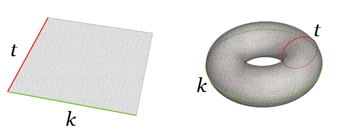
To compute the integral, we first make a change of variable

(8)x=k/2π,y=t/T,c=12π01dx01dy Ωxy

The integral is then written by virtue of the Stokes theorem as the line integral

(9)c2π=01dx Ax(x,0)+01dy Ay(1,y)01dxAx(x,1)01dyAy(0,y)

Because the region [0,1]×[0,1] is periodic, the berry connection at an opposite edges can only differ by a gauge transformation

(10)Ax(x,1)=Ax(x,0)θ(x)Ay(1,y)=Ay(0,y)ϕ(x)

which actually implies that

(11)u(x,1)=eiθ(x)u(x,0)u(1,y)=eiϕ(y)u(0,y)

where θ(x) and ϕ(y) are assumed to be smooth functions.

So

(12)c2π=θ(1)θ(0)ϕ(1)+ϕ(0)

At the same time, the phase the wavefunction gets by gets around the square region is

(13)eiθ(0)eiϕ(1)eiθ(1)eiϕ(0)u(0,0)

but since this is the same state as u(0,0), the single-valuedness (单值性) of the wavefunction requires

(14)θ(0)ϕ(1)+θ(1)+ϕ(0)=integer×2π

which means c must be an integer.

The physical interpretation of the above result is less exciting. It is like we are dragging the 1D crystal slowly at a constant speed, which gives a periodic H(t). After one period, the electron moves by one spatial period if it closely follow the lattice, which gives rise to a quantized number of electron transport. This is called adiabatic pumping, first proposed by David Thouless.

Nonetheless, the result is of great significance. We can state it very generally, that the integral of Berry curvature over a closed surface is an integer multiple of 2π.

The integer c is called the Chern number (陈数), after the Chinese geometer Shiing-Shen Chern (陈省身). This result is a special case of the Chern-Gauss-Bonnet theorem, for a 2D manifold (二维流形).

We will see later, this leads to more interesting phenomena in transport.


3. Electric polarization

Polarization in a finite system is easy to think about. For a periodic insulating system (a metal cannot sustain a polarization), this becomes mind-boggling.

polarization

In a first approach, we may write

(15)Psample=1Vsamplesampled3r rρ(r)

In order to use this definition, we need to assume a macroscopic but finite crystal. But the integral then has contributions from both the surface and the bulk regions, which cannot be easily disentangled. Moreover, if you construct a sample of size L×L×L, you may easily find a truncation where the surface change σ shifts from left to right, or vice versa. This leads to an uncertainty of the order σL3. So, this definition does not work.

The second approach can be formulated via

(16)Pcell=1Vcellcelld3r rρ(r)

Now you have no problem with the surfaces. But this This definition is also flawed, as it depends on the shape and location of the unit cell.

To understand the contribution of electrons to the polarization, we need the so-called modern theory of polarization, developed by Resta, King-Smith and Vanderbilt, and others. Think about the Maxwell equation, the current density of bound charges is

(17)j=Pt+×M

we will focus on the first term, for non-magnetic materials. So we see polarization P is really a quantity of change

(18)ΔP=t1t2dt1Vd3rj(r,t)

Notice that this is a current in process that incurs the polarization, without external fields, in an insulator. So it can only be the adiabatic current. And it is lattice periodic.

(19)ΔP=t1t2dt1Vcellcellj(r,t)

To make our lives easier, let's just carry out the calculation for a 1D system.

(20)ΔP=eat1t2dtBZdk2πΩkt=eaλ1λ2dλBZdk2πΩkλ=ieaλ1λ2dλBZdk2π(ukk|ukλc.c.)

Sketches

An simplification can be made if we introduce the Berry connection into the formula

(21)Ωkλ=AλkAkλ

In the periodic gauge, ψk+g=ψk

(22)eigr|uk+g, λ=|uk, λ

where the LHS and RHS are both periodic, as they should be. It follows then that A(k+g)=A(k) is also periodic in k, so the integral dkAλ=0. Then we have

(23)ΔP=P2P1

where

(24)Pi=eaBZdk2πAk(λi),i=1,2.

So, all of sudden we can define a Pi, as if it is a state function. But we have said, this is not possible. Indeed, there is a price in doing this. That is, it is defined only up to an integer multiple of ea, because as we choose the periodic gauge, we lose the track of the number of times the phase winds around in the BZ .

For example you can consider the polarization of a 1D crystal with inversion symmetry.

(25)P=P+nea

such that

(26)P=12nea

But it is only determined modulo
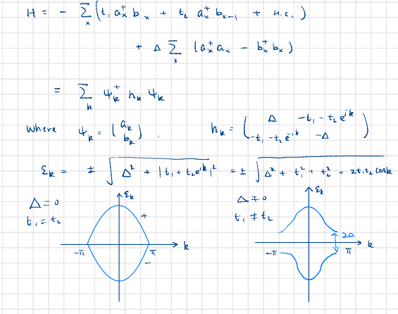
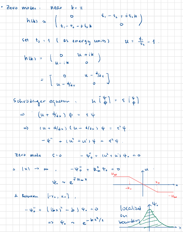
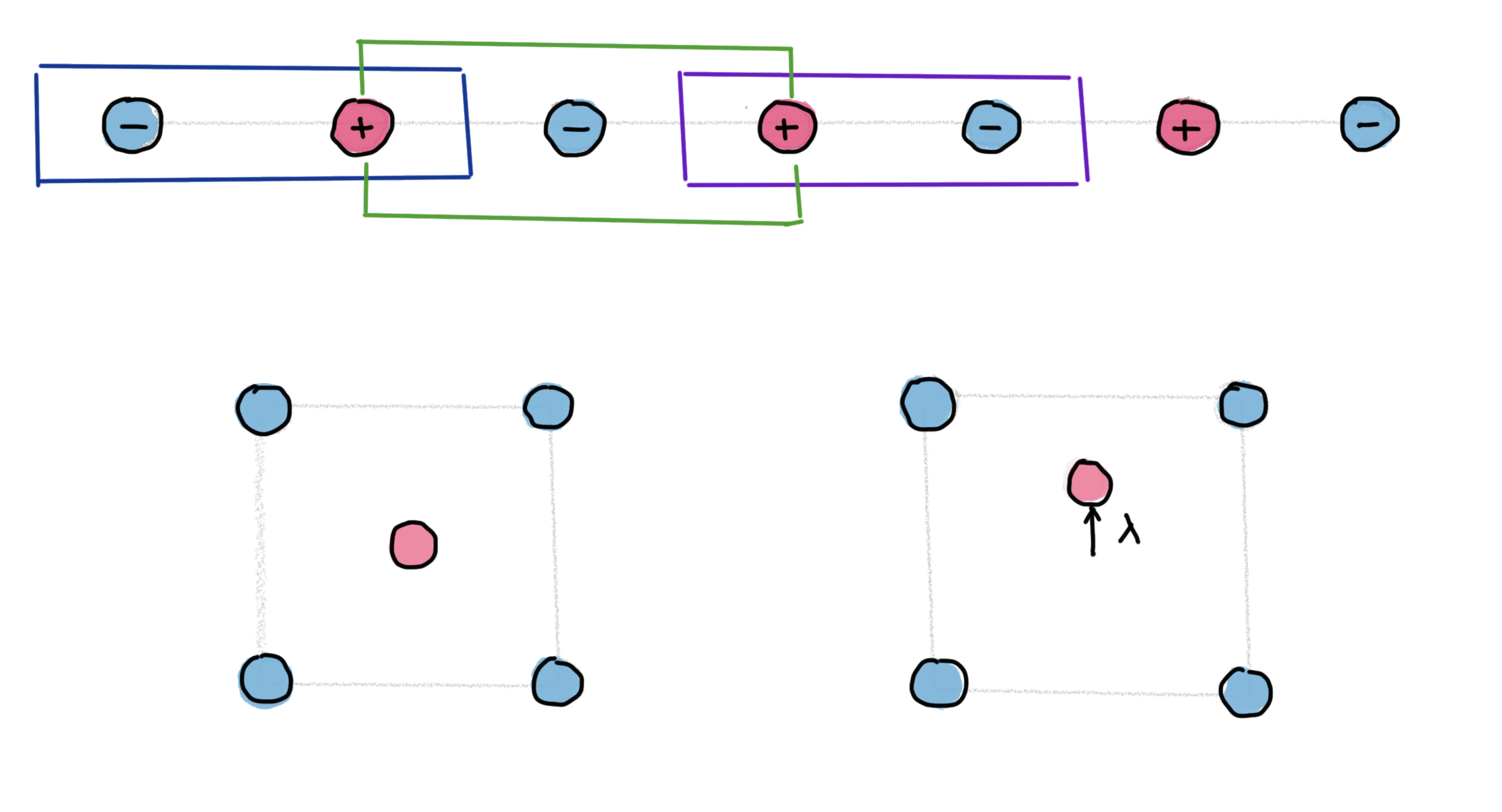
 ea, so P=0 or ea/2.


3. SSH model again

image-20230420115318567


image-20230420115342281

image-20230420115456895

image-20230420115534748

image-20230420115602275